> ## Documentation Index
> Fetch the complete documentation index at: https://nixtlaverse.nixtla.io/llms.txt
> Use this file to discover all available pages before exploring further.
# Intermittent Data
> In this notebook, we’ll implement models for intermittent or sparse
> data using the M5 dataset.
Intermittent or sparse data has very few non-zero observations. This
type of data is hard to forecast because the zero values increase the
uncertainty about the underlying patterns in the data. Furthermore, once
a non-zero observation occurs, there can be considerable variation in
its size. Intermittent time series are common in many industries,
including finance, retail, transportation, and energy. Given the
ubiquity of this type of series, special methods have been developed to
forecast them. The first was from [Croston (1972)](#ref), followed by
several variants and by different aggregation frameworks.
The models of
[NeuralForecast](https://nixtlaverse.nixtla.io/statsforecast/) can be
trained to model sparse or intermittent time series using a `Poisson`
distribution loss. By the end of this tutorial, you’ll have a good
understanding of these models and how to use them.
**Outline:**
1. Install libraries
2. Load and explore the data
3. Train models for intermittent data
4. Perform Cross Validation
> **Tip**
>
> You can use Colab to run this Notebook interactively
>
>
>  >
> **Warning**
>
> To reduce the computation time, it is recommended to use GPU. Using
> Colab, do not forget to activate it. Just go to
> `Runtime>Change runtime type` and select GPU as hardware accelerator.
## 1. Install libraries
We assume that you have NeuralForecast already installed. If not, check
this guide for instructions on [how to install
NeuralForecast](https://nixtlaverse.nixtla.io/neuralforecast/docs/getting-started/installation.html)
Install the necessary packages using `pip install neuralforecast`
```python theme={null}
%%capture
!pip install statsforecast s3fs fastparquet neuralforecast
```
## 2. Load and explore the data
For this example, we’ll use a subset of the [M5
Competition](https://www.sciencedirect.com/science/article/pii/S0169207021001187#:~:text=The%20objective%20of%20the%20M5,the%20uncertainty%20around%20these%20forecasts)
dataset. Each time series represents the unit sales of a particular
product in a given Walmart store. At this level (product-store), most of
the data is intermittent. We first need to import the data.
```python theme={null}
import pandas as pd
from utilsforecast.plotting import plot_series
```
```python theme={null}
Y_df = pd.read_parquet('https://m5-benchmarks.s3.amazonaws.com/data/train/target.parquet')
Y_df = Y_df.rename(columns={
'item_id': 'unique_id',
'timestamp': 'ds',
'demand': 'y'
})
Y_df['ds'] = pd.to_datetime(Y_df['ds'])
```
For simplicity sake we will keep just one category
```python theme={null}
Y_df = Y_df.query('unique_id.str.startswith("FOODS_3")')
Y_df['unique_id'] = Y_df['unique_id'].astype(str)
Y_df = Y_df.reset_index(drop=True)
```
Plot some series using the plot method from the `StatsForecast` class.
This method prints 8 random series from the dataset and is useful for
basic
[EDA](https://nixtlaverse.nixtla.io/statsforecast/src/core/core.html#statsforecast.plot).
```python theme={null}
plot_series(Y_df)
```
>
> **Warning**
>
> To reduce the computation time, it is recommended to use GPU. Using
> Colab, do not forget to activate it. Just go to
> `Runtime>Change runtime type` and select GPU as hardware accelerator.
## 1. Install libraries
We assume that you have NeuralForecast already installed. If not, check
this guide for instructions on [how to install
NeuralForecast](https://nixtlaverse.nixtla.io/neuralforecast/docs/getting-started/installation.html)
Install the necessary packages using `pip install neuralforecast`
```python theme={null}
%%capture
!pip install statsforecast s3fs fastparquet neuralforecast
```
## 2. Load and explore the data
For this example, we’ll use a subset of the [M5
Competition](https://www.sciencedirect.com/science/article/pii/S0169207021001187#:~:text=The%20objective%20of%20the%20M5,the%20uncertainty%20around%20these%20forecasts)
dataset. Each time series represents the unit sales of a particular
product in a given Walmart store. At this level (product-store), most of
the data is intermittent. We first need to import the data.
```python theme={null}
import pandas as pd
from utilsforecast.plotting import plot_series
```
```python theme={null}
Y_df = pd.read_parquet('https://m5-benchmarks.s3.amazonaws.com/data/train/target.parquet')
Y_df = Y_df.rename(columns={
'item_id': 'unique_id',
'timestamp': 'ds',
'demand': 'y'
})
Y_df['ds'] = pd.to_datetime(Y_df['ds'])
```
For simplicity sake we will keep just one category
```python theme={null}
Y_df = Y_df.query('unique_id.str.startswith("FOODS_3")')
Y_df['unique_id'] = Y_df['unique_id'].astype(str)
Y_df = Y_df.reset_index(drop=True)
```
Plot some series using the plot method from the `StatsForecast` class.
This method prints 8 random series from the dataset and is useful for
basic
[EDA](https://nixtlaverse.nixtla.io/statsforecast/src/core/core.html#statsforecast.plot).
```python theme={null}
plot_series(Y_df)
```
 ## 3. Train models for intermittent data
```python theme={null}
from ray import tune
from neuralforecast import NeuralForecast
from neuralforecast.auto import AutoNHITS, AutoTFT
from neuralforecast.losses.pytorch import DistributionLoss
```
Each `Auto` model contains a default search space that was extensively
tested on multiple large-scale datasets. Additionally, users can define
specific search spaces tailored for particular datasets and tasks.
First, we create a custom search space for the `AutoNHITS` and `AutoTFT`
models. Search spaces are specified with dictionaries, where keys
corresponds to the model’s hyperparameter and the value is a `Tune`
function to specify how the hyperparameter will be sampled. For example,
use `randint` to sample integers uniformly, and `choice` to sample
values of a list.
```python theme={null}
config_nhits = {
"input_size": tune.choice([28, 28*2, 28*3, 28*5]), # Length of input window
"n_blocks": 5*[1], # Length of input window
"mlp_units": 5 * [[512, 512]], # Length of input window
"n_pool_kernel_size": tune.choice([5*[1], 5*[2], 5*[4],
[8, 4, 2, 1, 1]]), # MaxPooling Kernel size
"n_freq_downsample": tune.choice([[8, 4, 2, 1, 1],
[1, 1, 1, 1, 1]]), # Interpolation expressivity ratios
"learning_rate": tune.loguniform(1e-4, 1e-2), # Initial Learning rate
"scaler_type": tune.choice([None]), # Scaler type
"max_steps": tune.choice([1000]), # Max number of training iterations
"batch_size": tune.choice([32, 64, 128, 256]), # Number of series in batch
"windows_batch_size": tune.choice([128, 256, 512, 1024]), # Number of windows in batch
"random_seed": tune.randint(1, 20), # Random seed
}
config_tft = {
"input_size": tune.choice([28, 28*2, 28*3]), # Length of input window
"hidden_size": tune.choice([64, 128, 256]), # Size of embeddings and encoders
"learning_rate": tune.loguniform(1e-4, 1e-2), # Initial learning rate
"scaler_type": tune.choice([None]), # Scaler type
"max_steps": tune.choice([500, 1000]), # Max number of training iterations
"batch_size": tune.choice([32, 64, 128, 256]), # Number of series in batch
"windows_batch_size": tune.choice([128, 256, 512, 1024]), # Number of windows in batch
"random_seed": tune.randint(1, 20), # Random seed
}
```
To instantiate an `Auto` model you need to define:
* `h`: forecasting horizon.
* `loss`: training and validation loss from
`neuralforecast.losses.pytorch`.
* `config`: hyperparameter search space. If `None`, the `Auto` class
will use a pre-defined suggested hyperparameter space.
* `search_alg`: search algorithm (from `tune.search`), default is
random search. Refer to
[https://docs.ray.io/en/latest/tune/api\_docs/suggestion.html](https://docs.ray.io/en/latest/tune/api_docs/suggestion.html) for more
information on the different search algorithm options.
* `num_samples`: number of configurations explored.
In this example we set horizon `h` as 28, use the `Poisson` distribution
loss (ideal for count data) for training and validation, and use the
default search algorithm.
```python theme={null}
nf = NeuralForecast(
models=[
AutoNHITS(h=28, config=config_nhits, loss=DistributionLoss(distribution='Poisson', level=[80, 90]), num_samples=5),
AutoTFT(h=28, config=config_tft, loss=DistributionLoss(distribution='Poisson', level=[80, 90]), num_samples=2),
],
freq='D'
)
```
> **Tip**
>
> The number of samples, `num_samples`, is a crucial parameter! Larger
> values will usually produce better results as we explore more
> configurations in the search space, but it will increase training
> times. Larger search spaces will usually require more samples. As a
> general rule, we recommend setting `num_samples` higher than 20.
Next, we use the `Neuralforecast` class to train the `Auto` model. In
this step, `Auto` models will automatically perform hyperparamter tuning
training multiple models with different hyperparameters, producing the
forecasts on the validation set, and evaluating them. The best
configuration is selected based on the error on a validation set. Only
the best model is stored and used during inference.
```python theme={null}
%%capture
nf.fit(df=Y_df)
```
Next, we use the `predict` method to forecast the next 28 days using the
optimal hyperparameters.
```python theme={null}
fcst_df = nf.predict()
```
```text theme={null}
GPU available: True (cuda), used: True
TPU available: False, using: 0 TPU cores
HPU available: False, using: 0 HPUs
LOCAL_RANK: 0 - CUDA_VISIBLE_DEVICES: [0]
GPU available: True (cuda), used: True
TPU available: False, using: 0 TPU cores
HPU available: False, using: 0 HPUs
LOCAL_RANK: 0 - CUDA_VISIBLE_DEVICES: [0]
```
```text theme={null}
Predicting: | | 0/? [00:00
## 4. Cross Validation
Time series cross-validation is a method for evaluating how a model
would have performed in the past. It works by defining a sliding window
across the historical data and predicting the period following it.
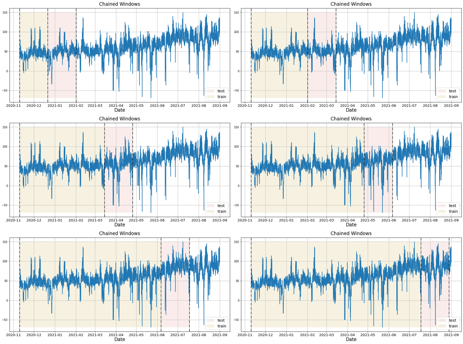
[NeuralForecast](https://nixtlaverse.nixtla.io/neuralforecast/) has an
implementation of time series cross-validation that is fast and easy to
use.
The `cross_validation` method from the `NeuralForecast` class takes the
following arguments.
* `df`: training data frame
* `step_size` (int): step size between each window. In other words:
how often do you want to run the forecasting processes.
* `n_windows` (int): number of windows used for cross validation. In
other words: what number of forecasting processes in the past do you
want to evaluate.
```python theme={null}
nf = NeuralForecast(
models=[
AutoNHITS(h=28, config=config_nhits, loss=DistributionLoss(distribution='Poisson', level=[80, 90]), num_samples=5),
AutoTFT(h=28, config=config_tft, loss=DistributionLoss(distribution='Poisson', level=[80, 90]), num_samples=2),
],
freq='D'
)
```
```python theme={null}
%%capture
cv_df = nf.cross_validation(Y_df, n_windows=3, step_size=28)
```
The `cv_df` object is a new data frame that includes the following
columns:
* `unique_id`: contains the id corresponding to the time series
* `ds`: datestamp or temporal index
* `cutoff`: the last datestamp or temporal index for the n\_windows. If
n\_windows=1, then one unique cuttoff value, if n\_windows=2 then two
unique cutoff values.
* `y`: true value
* `"model"`: columns with the model’s name and fitted value.
```python theme={null}
cv_df.head()
```
| | unique\_id | ds | cutoff | AutoNHITS | AutoNHITS-median | AutoNHITS-lo-90 | AutoNHITS-lo-80 | AutoNHITS-hi-80 | AutoNHITS-hi-90 | AutoTFT | AutoTFT-median | AutoTFT-lo-90 | AutoTFT-lo-80 | AutoTFT-hi-80 | AutoTFT-hi-90 | y |
| - | -------------------- | ---------- | ---------- | --------- | ---------------- | --------------- | --------------- | --------------- | --------------- | ------- | -------------- | ------------- | ------------- | ------------- | ------------- | --- |
| 0 | FOODS\_3\_001\_CA\_1 | 2016-02-29 | 2016-02-28 | 0.550 | 0.0 | 0.0 | 0.0 | 2.0 | 2.0 | 0.775 | 1.0 | 0.0 | 0.0 | 2.0 | 2.0 | 0.0 |
| 1 | FOODS\_3\_001\_CA\_1 | 2016-03-01 | 2016-02-28 | 0.611 | 0.0 | 0.0 | 0.0 | 2.0 | 2.0 | 0.746 | 1.0 | 0.0 | 0.0 | 2.0 | 2.0 | 1.0 |
| 2 | FOODS\_3\_001\_CA\_1 | 2016-03-02 | 2016-02-28 | 0.567 | 0.0 | 0.0 | 0.0 | 2.0 | 2.0 | 0.750 | 1.0 | 0.0 | 0.0 | 2.0 | 2.0 | 1.0 |
| 3 | FOODS\_3\_001\_CA\_1 | 2016-03-03 | 2016-02-28 | 0.554 | 0.0 | 0.0 | 0.0 | 2.0 | 2.0 | 0.750 | 1.0 | 0.0 | 0.0 | 2.0 | 2.0 | 0.0 |
| 4 | FOODS\_3\_001\_CA\_1 | 2016-03-04 | 2016-02-28 | 0.627 | 0.0 | 0.0 | 0.0 | 2.0 | 2.0 | 0.788 | 1.0 | 0.0 | 0.0 | 2.0 | 3.0 | 0.0 |
```python theme={null}
for cutoff in cv_df['cutoff'].unique():
display(plot_series(Y_df,
cv_df.query('cutoff == @cutoff').drop(columns=['cutoff', 'y', 'AutoNHITS-median', 'AutoTFT-median']),
max_insample_length=28*4,
ids=['FOODS_3_001_CA_1'],
level=[90]))
```
## 3. Train models for intermittent data
```python theme={null}
from ray import tune
from neuralforecast import NeuralForecast
from neuralforecast.auto import AutoNHITS, AutoTFT
from neuralforecast.losses.pytorch import DistributionLoss
```
Each `Auto` model contains a default search space that was extensively
tested on multiple large-scale datasets. Additionally, users can define
specific search spaces tailored for particular datasets and tasks.
First, we create a custom search space for the `AutoNHITS` and `AutoTFT`
models. Search spaces are specified with dictionaries, where keys
corresponds to the model’s hyperparameter and the value is a `Tune`
function to specify how the hyperparameter will be sampled. For example,
use `randint` to sample integers uniformly, and `choice` to sample
values of a list.
```python theme={null}
config_nhits = {
"input_size": tune.choice([28, 28*2, 28*3, 28*5]), # Length of input window
"n_blocks": 5*[1], # Length of input window
"mlp_units": 5 * [[512, 512]], # Length of input window
"n_pool_kernel_size": tune.choice([5*[1], 5*[2], 5*[4],
[8, 4, 2, 1, 1]]), # MaxPooling Kernel size
"n_freq_downsample": tune.choice([[8, 4, 2, 1, 1],
[1, 1, 1, 1, 1]]), # Interpolation expressivity ratios
"learning_rate": tune.loguniform(1e-4, 1e-2), # Initial Learning rate
"scaler_type": tune.choice([None]), # Scaler type
"max_steps": tune.choice([1000]), # Max number of training iterations
"batch_size": tune.choice([32, 64, 128, 256]), # Number of series in batch
"windows_batch_size": tune.choice([128, 256, 512, 1024]), # Number of windows in batch
"random_seed": tune.randint(1, 20), # Random seed
}
config_tft = {
"input_size": tune.choice([28, 28*2, 28*3]), # Length of input window
"hidden_size": tune.choice([64, 128, 256]), # Size of embeddings and encoders
"learning_rate": tune.loguniform(1e-4, 1e-2), # Initial learning rate
"scaler_type": tune.choice([None]), # Scaler type
"max_steps": tune.choice([500, 1000]), # Max number of training iterations
"batch_size": tune.choice([32, 64, 128, 256]), # Number of series in batch
"windows_batch_size": tune.choice([128, 256, 512, 1024]), # Number of windows in batch
"random_seed": tune.randint(1, 20), # Random seed
}
```
To instantiate an `Auto` model you need to define:
* `h`: forecasting horizon.
* `loss`: training and validation loss from
`neuralforecast.losses.pytorch`.
* `config`: hyperparameter search space. If `None`, the `Auto` class
will use a pre-defined suggested hyperparameter space.
* `search_alg`: search algorithm (from `tune.search`), default is
random search. Refer to
[https://docs.ray.io/en/latest/tune/api\_docs/suggestion.html](https://docs.ray.io/en/latest/tune/api_docs/suggestion.html) for more
information on the different search algorithm options.
* `num_samples`: number of configurations explored.
In this example we set horizon `h` as 28, use the `Poisson` distribution
loss (ideal for count data) for training and validation, and use the
default search algorithm.
```python theme={null}
nf = NeuralForecast(
models=[
AutoNHITS(h=28, config=config_nhits, loss=DistributionLoss(distribution='Poisson', level=[80, 90]), num_samples=5),
AutoTFT(h=28, config=config_tft, loss=DistributionLoss(distribution='Poisson', level=[80, 90]), num_samples=2),
],
freq='D'
)
```
> **Tip**
>
> The number of samples, `num_samples`, is a crucial parameter! Larger
> values will usually produce better results as we explore more
> configurations in the search space, but it will increase training
> times. Larger search spaces will usually require more samples. As a
> general rule, we recommend setting `num_samples` higher than 20.
Next, we use the `Neuralforecast` class to train the `Auto` model. In
this step, `Auto` models will automatically perform hyperparamter tuning
training multiple models with different hyperparameters, producing the
forecasts on the validation set, and evaluating them. The best
configuration is selected based on the error on a validation set. Only
the best model is stored and used during inference.
```python theme={null}
%%capture
nf.fit(df=Y_df)
```
Next, we use the `predict` method to forecast the next 28 days using the
optimal hyperparameters.
```python theme={null}
fcst_df = nf.predict()
```
```text theme={null}
GPU available: True (cuda), used: True
TPU available: False, using: 0 TPU cores
HPU available: False, using: 0 HPUs
LOCAL_RANK: 0 - CUDA_VISIBLE_DEVICES: [0]
GPU available: True (cuda), used: True
TPU available: False, using: 0 TPU cores
HPU available: False, using: 0 HPUs
LOCAL_RANK: 0 - CUDA_VISIBLE_DEVICES: [0]
```
```text theme={null}
Predicting: | | 0/? [00:00
## 4. Cross Validation
Time series cross-validation is a method for evaluating how a model
would have performed in the past. It works by defining a sliding window
across the historical data and predicting the period following it.

[NeuralForecast](https://nixtlaverse.nixtla.io/neuralforecast/) has an
implementation of time series cross-validation that is fast and easy to
use.
The `cross_validation` method from the `NeuralForecast` class takes the
following arguments.
* `df`: training data frame
* `step_size` (int): step size between each window. In other words:
how often do you want to run the forecasting processes.
* `n_windows` (int): number of windows used for cross validation. In
other words: what number of forecasting processes in the past do you
want to evaluate.
```python theme={null}
nf = NeuralForecast(
models=[
AutoNHITS(h=28, config=config_nhits, loss=DistributionLoss(distribution='Poisson', level=[80, 90]), num_samples=5),
AutoTFT(h=28, config=config_tft, loss=DistributionLoss(distribution='Poisson', level=[80, 90]), num_samples=2),
],
freq='D'
)
```
```python theme={null}
%%capture
cv_df = nf.cross_validation(Y_df, n_windows=3, step_size=28)
```
The `cv_df` object is a new data frame that includes the following
columns:
* `unique_id`: contains the id corresponding to the time series
* `ds`: datestamp or temporal index
* `cutoff`: the last datestamp or temporal index for the n\_windows. If
n\_windows=1, then one unique cuttoff value, if n\_windows=2 then two
unique cutoff values.
* `y`: true value
* `"model"`: columns with the model’s name and fitted value.
```python theme={null}
cv_df.head()
```
| | unique\_id | ds | cutoff | AutoNHITS | AutoNHITS-median | AutoNHITS-lo-90 | AutoNHITS-lo-80 | AutoNHITS-hi-80 | AutoNHITS-hi-90 | AutoTFT | AutoTFT-median | AutoTFT-lo-90 | AutoTFT-lo-80 | AutoTFT-hi-80 | AutoTFT-hi-90 | y |
| - | -------------------- | ---------- | ---------- | --------- | ---------------- | --------------- | --------------- | --------------- | --------------- | ------- | -------------- | ------------- | ------------- | ------------- | ------------- | --- |
| 0 | FOODS\_3\_001\_CA\_1 | 2016-02-29 | 2016-02-28 | 0.550 | 0.0 | 0.0 | 0.0 | 2.0 | 2.0 | 0.775 | 1.0 | 0.0 | 0.0 | 2.0 | 2.0 | 0.0 |
| 1 | FOODS\_3\_001\_CA\_1 | 2016-03-01 | 2016-02-28 | 0.611 | 0.0 | 0.0 | 0.0 | 2.0 | 2.0 | 0.746 | 1.0 | 0.0 | 0.0 | 2.0 | 2.0 | 1.0 |
| 2 | FOODS\_3\_001\_CA\_1 | 2016-03-02 | 2016-02-28 | 0.567 | 0.0 | 0.0 | 0.0 | 2.0 | 2.0 | 0.750 | 1.0 | 0.0 | 0.0 | 2.0 | 2.0 | 1.0 |
| 3 | FOODS\_3\_001\_CA\_1 | 2016-03-03 | 2016-02-28 | 0.554 | 0.0 | 0.0 | 0.0 | 2.0 | 2.0 | 0.750 | 1.0 | 0.0 | 0.0 | 2.0 | 2.0 | 0.0 |
| 4 | FOODS\_3\_001\_CA\_1 | 2016-03-04 | 2016-02-28 | 0.627 | 0.0 | 0.0 | 0.0 | 2.0 | 2.0 | 0.788 | 1.0 | 0.0 | 0.0 | 2.0 | 3.0 | 0.0 |
```python theme={null}
for cutoff in cv_df['cutoff'].unique():
display(plot_series(Y_df,
cv_df.query('cutoff == @cutoff').drop(columns=['cutoff', 'y', 'AutoNHITS-median', 'AutoTFT-median']),
max_insample_length=28*4,
ids=['FOODS_3_001_CA_1'],
level=[90]))
```


 ### Evaluate
In this section we will evaluate the performance of each model each
cross validation window using the MSE metric.
```python theme={null}
from utilsforecast.losses import mse, mae
from utilsforecast.evaluation import evaluate
```
```python theme={null}
metrics = pd.DataFrame()
for cutoff in cv_df["cutoff"].unique():
metrics_per_cutoff = evaluate(cv_df.query("cutoff == @cutoff"),
metrics=[mse, mae],
models=['AutoNHITS', 'AutoTFT'],
level=[80, 90],
agg_fn="mean")
metrics_per_cutoff = metrics_per_cutoff.assign(cutoff=cutoff)
metrics = pd.concat([metrics, metrics_per_cutoff])
metrics
```
| | metric | AutoNHITS | AutoTFT | cutoff |
| - | ------ | --------- | --------- | ---------- |
| 0 | mse | 10.059308 | 10.909020 | 2016-02-28 |
| 1 | mae | 1.485914 | 1.554572 | 2016-02-28 |
| 0 | mse | 9.590549 | 10.253903 | 2016-03-27 |
| 1 | mae | 1.494229 | 1.561868 | 2016-03-27 |
| 0 | mse | 9.596170 | 10.300666 | 2016-04-24 |
| 1 | mae | 1.501949 | 1.564157 | 2016-04-24 |
## References
* [Croston, J. D. (1972). Forecasting and stock control for
intermittent demands. Journal of the Operational Research Society,
23(3),
289-303.](https://link.springer.com/article/10.1057/jors.1972.50)
* [Cristian Challu, Kin G. Olivares, Boris N. Oreshkin, Federico
Garza, Max Mergenthaler-Canseco, Artur Dubrawski (2021). N-HiTS:
Neural Hierarchical Interpolation for Time Series Forecasting.
Accepted at AAAI 2023.](https://arxiv.org/abs/2201.12886)
### Evaluate
In this section we will evaluate the performance of each model each
cross validation window using the MSE metric.
```python theme={null}
from utilsforecast.losses import mse, mae
from utilsforecast.evaluation import evaluate
```
```python theme={null}
metrics = pd.DataFrame()
for cutoff in cv_df["cutoff"].unique():
metrics_per_cutoff = evaluate(cv_df.query("cutoff == @cutoff"),
metrics=[mse, mae],
models=['AutoNHITS', 'AutoTFT'],
level=[80, 90],
agg_fn="mean")
metrics_per_cutoff = metrics_per_cutoff.assign(cutoff=cutoff)
metrics = pd.concat([metrics, metrics_per_cutoff])
metrics
```
| | metric | AutoNHITS | AutoTFT | cutoff |
| - | ------ | --------- | --------- | ---------- |
| 0 | mse | 10.059308 | 10.909020 | 2016-02-28 |
| 1 | mae | 1.485914 | 1.554572 | 2016-02-28 |
| 0 | mse | 9.590549 | 10.253903 | 2016-03-27 |
| 1 | mae | 1.494229 | 1.561868 | 2016-03-27 |
| 0 | mse | 9.596170 | 10.300666 | 2016-04-24 |
| 1 | mae | 1.501949 | 1.564157 | 2016-04-24 |
## References
* [Croston, J. D. (1972). Forecasting and stock control for
intermittent demands. Journal of the Operational Research Society,
23(3),
289-303.](https://link.springer.com/article/10.1057/jors.1972.50)
* [Cristian Challu, Kin G. Olivares, Boris N. Oreshkin, Federico
Garza, Max Mergenthaler-Canseco, Artur Dubrawski (2021). N-HiTS:
Neural Hierarchical Interpolation for Time Series Forecasting.
Accepted at AAAI 2023.](https://arxiv.org/abs/2201.12886)