> ## Documentation Index
> Fetch the complete documentation index at: https://nixtlaverse.nixtla.io/llms.txt
> Use this file to discover all available pages before exploring further.
# Forecasting with TFT: Temporal Fusion Transformer
Temporal Fusion Transformer (TFT) proposed by Lim et al. \[1] is one of
the most popular transformer-based model for time-series forecasting. In
summary, TFT combines gating layers, an LSTM recurrent encoder, with
multi-head attention layers for a multi-step forecasting strategy
decoder. For more details on the Nixtla’s TFT implementation visit [this
link](https://nixtlaverse.nixtla.io/neuralforecast/models.tft.html).
In this notebook we show how to train the TFT model on the Texas
electricity market load data (ERCOT). Accurately forecasting electricity
markets is of great interest, as it is useful for planning distribution
and consumption.
We will show you how to load the data, train the TFT performing
automatic hyperparameter tuning, and produce forecasts. Then, we will
show you how to perform multiple historical forecasts for cross
validation.
You can run these experiments using GPU with Google Colab.
 ## 1. Libraries
```python theme={null}
%%capture
!pip install neuralforecast
```
```python theme={null}
import pandas as pd
```
## 2. Load ERCOT Data
The input to NeuralForecast is always a data frame in [long
format](https://www.theanalysisfactor.com/wide-and-long-data/) with
three columns: `unique_id`, `ds` and `y`:
* The `unique_id` (string, int or category) represents an identifier
for the series.
* The `ds` (datestamp or int) column should be either an integer
indexing time or a datestamp ideally like YYYY-MM-DD for a date or
YYYY-MM-DD HH:MM:SS for a timestamp.
* The `y` (numeric) represents the measurement we wish to forecast. We
will rename the
First, read the 2022 historic total demand of the ERCOT market. We
processed the original data (available
[here](https://www.ercot.com/gridinfo/load/load_hist)), by adding the
missing hour due to daylight saving time, parsing the date to datetime
format, and filtering columns of interest.
```python theme={null}
Y_df = pd.read_csv('https://datasets-nixtla.s3.amazonaws.com/ERCOT-clean.csv')
Y_df['ds'] = pd.to_datetime(Y_df['ds'])
Y_df.head()
```
| | unique\_id | ds | y |
| - | ---------- | ------------------- | ------------ |
| 0 | ERCOT | 2021-01-01 00:00:00 | 43719.849616 |
| 1 | ERCOT | 2021-01-01 01:00:00 | 43321.050347 |
| 2 | ERCOT | 2021-01-01 02:00:00 | 43063.067063 |
| 3 | ERCOT | 2021-01-01 03:00:00 | 43090.059203 |
| 4 | ERCOT | 2021-01-01 04:00:00 | 43486.590073 |
## 3. Model training and forecast
First, instantiate the `AutoTFT` model. The `AutoTFT` class will
automatically perform hyperparamter tunning using [Tune
library](https://docs.ray.io/en/latest/tune/index.html), exploring a
user-defined or default search space. Models are selected based on the
error on a validation set and the best model is then stored and used
during inference.
To instantiate `AutoTFT` you need to define:
* `h`: forecasting horizon
* `loss`: training loss
* `config`: hyperparameter search space. If `None`, the `AutoTFT`
class will use a pre-defined suggested hyperparameter space.
* `num_samples`: number of configurations explored.
```python theme={null}
from ray import tune
from neuralforecast.auto import AutoTFT
from neuralforecast.core import NeuralForecast
from neuralforecast.losses.pytorch import MAE
import logging
logging.getLogger("pytorch_lightning").setLevel(logging.WARNING)
```
> **Tip**
>
> Increase the `num_samples` parameter to explore a wider set of
> configurations for the selected models. As a rule of thumb choose it
> to be bigger than `15`.
>
> With `num_samples=3` this example should run in around 20 minutes.
```python theme={null}
horizon = 24
models = [AutoTFT(h=horizon,
loss=MAE(),
config=None,
num_samples=3)]
```
> **Tip**
>
> All our models can be used for both point and probabilistic
> forecasting. For producing probabilistic outputs, simply modify the
> loss to one of our `DistributionLoss`. The complete list of losses is
> available in [this
> link](https://nixtlaverse.nixtla.io/neuralforecast/losses.pytorch.html)
> **Important**
>
> TFT is a very large model and can require a lot of memory! If you are
> running out of GPU memory, try declaring your config search space and
> decrease the `hidden_size`, `n_heads`, and `windows_batch_size`
> parameters.
>
> This are all the parameters of the config:
>
> ```python theme={null}
> config = {
> "input_size": tune.choice([horizon]),
> "hidden_size": tune.choice([32]),
> "n_head": tune.choice([2]),
> "learning_rate": tune.loguniform(1e-4, 1e-1),
> "scaler_type": tune.choice(['robust', 'standard']),
> "max_steps": tune.choice([500, 1000]),
> "windows_batch_size": tune.choice([32]),
> "check_val_every_n_epoch": tune.choice([100]),
> "random_seed": tune.randint(1, 20),
> }
> ```
The `NeuralForecast` class has built-in methods to simplify the
forecasting pipelines, such as `fit`, `predit`, and `cross_validation`.
Instantiate a `NeuralForecast` object with the following required
parameters:
* `models`: a list of models.
* `freq`: a string indicating the frequency of the data. (See [panda’s
available
frequencies](https://pandas.pydata.org/pandas-docs/stable/user_guide/timeseries.html#offset-aliases).)
Then, use the `fit` method to train the `AutoTFT` model on the ERCOT
data. The total training time will depend on the hardware and the
explored configurations, it should take between 10 and 30 minutes.
```python theme={null}
%%capture
nf = NeuralForecast(
models=models,
freq='h')
nf.fit(df=Y_df)
```
Finally, use the `predict` method to forecast the next 24 hours after
the training data and plot the forecasts.
```python theme={null}
Y_hat_df = nf.predict()
Y_hat_df.head()
```
```text theme={null}
c:\Users\ospra\miniconda3\envs\neuralforecast\lib\site-packages\utilsforecast\processing.py:384: FutureWarning: 'H' is deprecated and will be removed in a future version, please use 'h' instead.
freq = pd.tseries.frequencies.to_offset(freq)
c:\Users\ospra\miniconda3\envs\neuralforecast\lib\site-packages\utilsforecast\processing.py:440: FutureWarning: 'H' is deprecated and will be removed in a future version, please use 'h' instead.
freq = pd.tseries.frequencies.to_offset(freq)
```
```text theme={null}
Predicting: | | 0/? [00:00
## 4. Cross validation for multiple historic forecasts
The `cross_validation` method allows you to simulate multiple historic
forecasts, greatly simplifying pipelines by replacing for loops with
`fit` and `predict` methods. See [this
tutorial](https://nixtlaverse.nixtla.io/statsforecast/docs/getting-started/getting_started_complete.html)
for an animation of how the windows are defined.
With time series data, cross validation is done by defining a sliding
window across the historical data and predicting the period following
it. This form of cross validation allows us to arrive at a better
estimation of our model’s predictive abilities across a wider range of
temporal instances while also keeping the data in the training set
contiguous as is required by our models. The `cross_validation` method
will use the validation set for hyperparameter selection, and will then
produce the forecasts for the test set.
Use the `cross_validation` method to produce all the daily forecasts for
September. Set the validation and test sizes. To produce daily forecasts
set the forecasting set the step size between windows as 24, to only
produce one forecast per day.
```python theme={null}
%%capture
val_size = 90*24 # 90 days x 24 hours
test_size = 30*24 # 30 days x 24 hours
fcst_df = nf.cross_validation(df=Y_df, val_size=val_size, test_size=test_size,
n_windows=None, step_size=horizon)
```
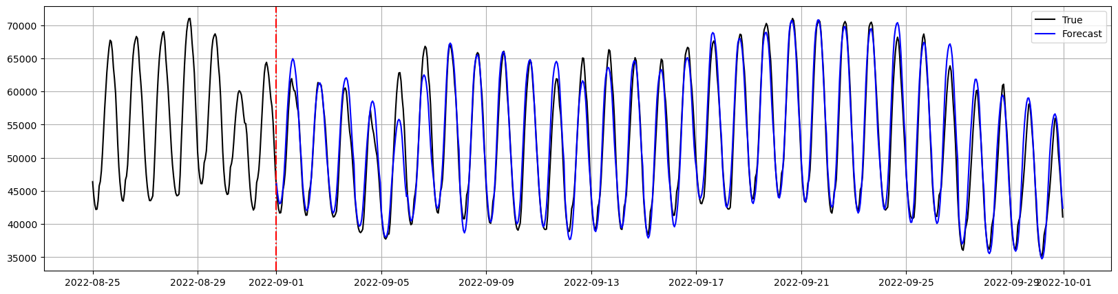
Finally, we merge the forecasts with the `Y_df` dataset and plot the
forecasts.
```python theme={null}
Y_hat_df = fcst_df.reset_index(drop=True)
Y_hat_df = Y_hat_df.drop(columns=['y','cutoff'])
```
```python theme={null}
plot_df = Y_df.merge(Y_hat_df, on=['unique_id','ds'], how='outer').tail(test_size+24*7)
plt.figure(figsize=(20,5))
plt.plot(plot_df['ds'], plot_df['y'], c='black', label='True')
plt.plot(plot_df['ds'], plot_df['AutoTFT'], c='blue', label='Forecast')
plt.axvline(pd.to_datetime('2022-09-01'), color='red', linestyle='-.')
plt.legend()
plt.grid()
plt.plot()
```
## 1. Libraries
```python theme={null}
%%capture
!pip install neuralforecast
```
```python theme={null}
import pandas as pd
```
## 2. Load ERCOT Data
The input to NeuralForecast is always a data frame in [long
format](https://www.theanalysisfactor.com/wide-and-long-data/) with
three columns: `unique_id`, `ds` and `y`:
* The `unique_id` (string, int or category) represents an identifier
for the series.
* The `ds` (datestamp or int) column should be either an integer
indexing time or a datestamp ideally like YYYY-MM-DD for a date or
YYYY-MM-DD HH:MM:SS for a timestamp.
* The `y` (numeric) represents the measurement we wish to forecast. We
will rename the
First, read the 2022 historic total demand of the ERCOT market. We
processed the original data (available
[here](https://www.ercot.com/gridinfo/load/load_hist)), by adding the
missing hour due to daylight saving time, parsing the date to datetime
format, and filtering columns of interest.
```python theme={null}
Y_df = pd.read_csv('https://datasets-nixtla.s3.amazonaws.com/ERCOT-clean.csv')
Y_df['ds'] = pd.to_datetime(Y_df['ds'])
Y_df.head()
```
| | unique\_id | ds | y |
| - | ---------- | ------------------- | ------------ |
| 0 | ERCOT | 2021-01-01 00:00:00 | 43719.849616 |
| 1 | ERCOT | 2021-01-01 01:00:00 | 43321.050347 |
| 2 | ERCOT | 2021-01-01 02:00:00 | 43063.067063 |
| 3 | ERCOT | 2021-01-01 03:00:00 | 43090.059203 |
| 4 | ERCOT | 2021-01-01 04:00:00 | 43486.590073 |
## 3. Model training and forecast
First, instantiate the `AutoTFT` model. The `AutoTFT` class will
automatically perform hyperparamter tunning using [Tune
library](https://docs.ray.io/en/latest/tune/index.html), exploring a
user-defined or default search space. Models are selected based on the
error on a validation set and the best model is then stored and used
during inference.
To instantiate `AutoTFT` you need to define:
* `h`: forecasting horizon
* `loss`: training loss
* `config`: hyperparameter search space. If `None`, the `AutoTFT`
class will use a pre-defined suggested hyperparameter space.
* `num_samples`: number of configurations explored.
```python theme={null}
from ray import tune
from neuralforecast.auto import AutoTFT
from neuralforecast.core import NeuralForecast
from neuralforecast.losses.pytorch import MAE
import logging
logging.getLogger("pytorch_lightning").setLevel(logging.WARNING)
```
> **Tip**
>
> Increase the `num_samples` parameter to explore a wider set of
> configurations for the selected models. As a rule of thumb choose it
> to be bigger than `15`.
>
> With `num_samples=3` this example should run in around 20 minutes.
```python theme={null}
horizon = 24
models = [AutoTFT(h=horizon,
loss=MAE(),
config=None,
num_samples=3)]
```
> **Tip**
>
> All our models can be used for both point and probabilistic
> forecasting. For producing probabilistic outputs, simply modify the
> loss to one of our `DistributionLoss`. The complete list of losses is
> available in [this
> link](https://nixtlaverse.nixtla.io/neuralforecast/losses.pytorch.html)
> **Important**
>
> TFT is a very large model and can require a lot of memory! If you are
> running out of GPU memory, try declaring your config search space and
> decrease the `hidden_size`, `n_heads`, and `windows_batch_size`
> parameters.
>
> This are all the parameters of the config:
>
> ```python theme={null}
> config = {
> "input_size": tune.choice([horizon]),
> "hidden_size": tune.choice([32]),
> "n_head": tune.choice([2]),
> "learning_rate": tune.loguniform(1e-4, 1e-1),
> "scaler_type": tune.choice(['robust', 'standard']),
> "max_steps": tune.choice([500, 1000]),
> "windows_batch_size": tune.choice([32]),
> "check_val_every_n_epoch": tune.choice([100]),
> "random_seed": tune.randint(1, 20),
> }
> ```
The `NeuralForecast` class has built-in methods to simplify the
forecasting pipelines, such as `fit`, `predit`, and `cross_validation`.
Instantiate a `NeuralForecast` object with the following required
parameters:
* `models`: a list of models.
* `freq`: a string indicating the frequency of the data. (See [panda’s
available
frequencies](https://pandas.pydata.org/pandas-docs/stable/user_guide/timeseries.html#offset-aliases).)
Then, use the `fit` method to train the `AutoTFT` model on the ERCOT
data. The total training time will depend on the hardware and the
explored configurations, it should take between 10 and 30 minutes.
```python theme={null}
%%capture
nf = NeuralForecast(
models=models,
freq='h')
nf.fit(df=Y_df)
```
Finally, use the `predict` method to forecast the next 24 hours after
the training data and plot the forecasts.
```python theme={null}
Y_hat_df = nf.predict()
Y_hat_df.head()
```
```text theme={null}
c:\Users\ospra\miniconda3\envs\neuralforecast\lib\site-packages\utilsforecast\processing.py:384: FutureWarning: 'H' is deprecated and will be removed in a future version, please use 'h' instead.
freq = pd.tseries.frequencies.to_offset(freq)
c:\Users\ospra\miniconda3\envs\neuralforecast\lib\site-packages\utilsforecast\processing.py:440: FutureWarning: 'H' is deprecated and will be removed in a future version, please use 'h' instead.
freq = pd.tseries.frequencies.to_offset(freq)
```
```text theme={null}
Predicting: | | 0/? [00:00
## 4. Cross validation for multiple historic forecasts
The `cross_validation` method allows you to simulate multiple historic
forecasts, greatly simplifying pipelines by replacing for loops with
`fit` and `predict` methods. See [this
tutorial](https://nixtlaverse.nixtla.io/statsforecast/docs/getting-started/getting_started_complete.html)
for an animation of how the windows are defined.
With time series data, cross validation is done by defining a sliding
window across the historical data and predicting the period following
it. This form of cross validation allows us to arrive at a better
estimation of our model’s predictive abilities across a wider range of
temporal instances while also keeping the data in the training set
contiguous as is required by our models. The `cross_validation` method
will use the validation set for hyperparameter selection, and will then
produce the forecasts for the test set.
Use the `cross_validation` method to produce all the daily forecasts for
September. Set the validation and test sizes. To produce daily forecasts
set the forecasting set the step size between windows as 24, to only
produce one forecast per day.
```python theme={null}
%%capture
val_size = 90*24 # 90 days x 24 hours
test_size = 30*24 # 30 days x 24 hours
fcst_df = nf.cross_validation(df=Y_df, val_size=val_size, test_size=test_size,
n_windows=None, step_size=horizon)
```
Finally, we merge the forecasts with the `Y_df` dataset and plot the
forecasts.
```python theme={null}
Y_hat_df = fcst_df.reset_index(drop=True)
Y_hat_df = Y_hat_df.drop(columns=['y','cutoff'])
```
```python theme={null}
plot_df = Y_df.merge(Y_hat_df, on=['unique_id','ds'], how='outer').tail(test_size+24*7)
plt.figure(figsize=(20,5))
plt.plot(plot_df['ds'], plot_df['y'], c='black', label='True')
plt.plot(plot_df['ds'], plot_df['AutoTFT'], c='blue', label='Forecast')
plt.axvline(pd.to_datetime('2022-09-01'), color='red', linestyle='-.')
plt.legend()
plt.grid()
plt.plot()
```
 ## Next Steps
In Challu et al \[2] we demonstrate that the N-HiTS model outperforms
the latest transformers by more than 20% with 50 times less computation.
Learn how to use the N-HiTS and the NeuralForecast library in [this
tutorial](../use-cases/electricity_peak_forecasting.html).
## References
\[1] [Lim, B., Arık, S. Ö., Loeff, N., & Pfister, T. (2021). Temporal
fusion transformers for interpretable multi-horizon time series
forecasting. International Journal of Forecasting, 37(4),
1748-1764.](https://www.sciencedirect.com/science/article/pii/S0169207021000637).
\[2] [Cristian Challu, Kin G. Olivares, Boris N. Oreshkin, Federico
Garza, Max Mergenthaler-Canseco, Artur Dubrawski (2021). N-HiTS: Neural
Hierarchical Interpolation for Time Series Forecasting. Accepted at AAAI
2023.](https://arxiv.org/abs/2201.12886)
## Next Steps
In Challu et al \[2] we demonstrate that the N-HiTS model outperforms
the latest transformers by more than 20% with 50 times less computation.
Learn how to use the N-HiTS and the NeuralForecast library in [this
tutorial](../use-cases/electricity_peak_forecasting.html).
## References
\[1] [Lim, B., Arık, S. Ö., Loeff, N., & Pfister, T. (2021). Temporal
fusion transformers for interpretable multi-horizon time series
forecasting. International Journal of Forecasting, 37(4),
1748-1764.](https://www.sciencedirect.com/science/article/pii/S0169207021000637).
\[2] [Cristian Challu, Kin G. Olivares, Boris N. Oreshkin, Federico
Garza, Max Mergenthaler-Canseco, Artur Dubrawski (2021). N-HiTS: Neural
Hierarchical Interpolation for Time Series Forecasting. Accepted at AAAI
2023.](https://arxiv.org/abs/2201.12886)