> ## Documentation Index
> Fetch the complete documentation index at: https://nixtlaverse.nixtla.io/llms.txt
> Use this file to discover all available pages before exploring further.
# Time Series Scaling
Scaling time series data is an important preprocessing step when using
neural forecasting methods for several reasons:
1. **Convergence speed**: Neural forecasting models tend to converge
faster when the features are on a similar scale.
2. **Avoiding vanishing or exploding gradients**: some architectures,
such as recurrent neural networks (RNNs), are sensitive to the scale
of input data. If the input values are too large, it could lead to
exploding gradients, where the gradients become too large and the
model becomes unstable. Conversely, very small input values could
lead to vanishing gradients, where weight updates during training
are negligible and the training fails to converge.
3. **Ensuring consistent scale**: Neural forecasting models have shared
global parameters for the all time series of the task. In cases
where time series have different scale, scaling ensures that no
particular time series dominates the learning process.
4. **Improving generalization**: time series with consistent scale can
lead to smoother loss surfaces. Moreover, scaling helps to
homogenize the distribution of the input data, which can also
improve generalization by avoiding out-of-range values.
The `Neuralforecast` library integrates two types of temporal scaling:
* **Time Series Scaling**: scaling each time series using all its data
on the train set before start training the model. This is done by
using the `local_scaler_type` parameter of the `Neuralforecast` core
class.
* **Window scaling (TemporalNorm)**: scaling each input window
separetly for each element of the batch at every training iteration.
This is done by using the `scaler_type` parameter of each model
class.
In this notebook, we will demonstrate how to scale the time series data
with both methods on an Eletricity Price Forecasting (EPF) task.
You can run these experiments using GPU with Google Colab.
 ## 1. Install `Neuralforecast`
```python theme={null}
%%capture
!pip install neuralforecast
!pip install hyperopt
```
## 2. Load Data
The `df` dataframe contains the target and exogenous variables past
information to train the model. The `unique_id` column identifies the
markets, `ds` contains the datestamps, and `y` the electricity price.
For future variables, we include a forecast of how much electricity will
be produced (`gen_forecast`), and day of week (`week_day`). Both the
electricity system demand and offer impact the price significantly,
including these variables to the model greatly improve performance, as
we demonstrate in Olivares et al. (2022).
The `futr_df` dataframe includes the information of the future exogenous
variables for the period we want to forecast (in this case, 24 hours
after the end of the train dataset `df`).
```python theme={null}
import pandas as pd
import matplotlib.pyplot as plt
```
```python theme={null}
df = pd.read_csv(
'https://datasets-nixtla.s3.amazonaws.com/EPF_FR_BE.csv',
parse_dates=['ds'],
)
futr_df = pd.read_csv(
'https://datasets-nixtla.s3.amazonaws.com/EPF_FR_BE_futr.csv',
parse_dates=['ds'],
)
df.head()
```
| | unique\_id | ds | y | gen\_forecast | system\_load | week\_day |
| - | ---------- | ------------------- | ----- | ------------- | ------------ | --------- |
| 0 | FR | 2015-01-01 00:00:00 | 53.48 | 76905.0 | 74812.0 | 3 |
| 1 | FR | 2015-01-01 01:00:00 | 51.93 | 75492.0 | 71469.0 | 3 |
| 2 | FR | 2015-01-01 02:00:00 | 48.76 | 74394.0 | 69642.0 | 3 |
| 3 | FR | 2015-01-01 03:00:00 | 42.27 | 72639.0 | 66704.0 | 3 |
| 4 | FR | 2015-01-01 04:00:00 | 38.41 | 69347.0 | 65051.0 | 3 |
We can see that `y` and the exogenous variables are on largely different
scales. Next, we show two methods to scale the data.
## 3. Time Series Scaling with `Neuralforecast` class
One of the most widely used approches for scaling time series is to
treat it as a pre-processing step, where each time series and temporal
exogenous variables are scaled based on their entire information in the
train set. Models are then trained on the scaled data.
To simplify pipelines, we added a scaling functionality to the
`Neuralforecast` class. Each time series will be scaled before training
the model with either `fit` or `cross_validation`, and scaling
statistics are stored. The class then uses the stored statistics to
scale the forecasts back to the original scale before returning the
forecasts.
### 3.a. Instantiate model and `Neuralforecast` class
In this example we will use the `TimesNet` model, recently proposed in
[Wu, Haixu, et al. (2022)](https://arxiv.org/abs/2210.02186). First
instantiate the model with the desired parameters.
```python theme={null}
import logging
from neuralforecast.models import TimesNet
from neuralforecast.core import NeuralForecast
```
```python theme={null}
logging.getLogger("pytorch_lightning").setLevel(logging.WARNING)
```
```python theme={null}
horizon = 24 # day-ahead daily forecast
model = TimesNet(h = horizon, # Horizon
input_size = 5*horizon, # Length of input window
max_steps = 100, # Training iterations
top_k = 3, # Number of periods (for FFT).
num_kernels = 3, # Number of kernels for Inception module
batch_size = 2, # Number of time series per batch
windows_batch_size = 32, # Number of windows per batch
learning_rate = 0.001, # Learning rate
futr_exog_list = ['gen_forecast', 'week_day'], # Future exogenous variables
scaler_type = None) # We use the Core scaling method
```
```text theme={null}
Seed set to 1
```
Fit the model by instantiating a `NeuralForecast` object and using the
`fit` method. The `local_scaler_type` parameter is used to specify the
type of scaling to be used. In this case, we will use `standard`, which
scales the data to have zero mean and unit variance.Other supported
scalers are `minmax`, `robust`, `robust-iqr`, `minmax`, and `boxcox`.
```python theme={null}
nf = NeuralForecast(models=[model], freq='h', local_scaler_type='standard')
nf.fit(df=df)
```
```text theme={null}
Sanity Checking: | …
```
```text theme={null}
Training: | …
```
```text theme={null}
Validation: | …
```
### 3.b Forecast and plots
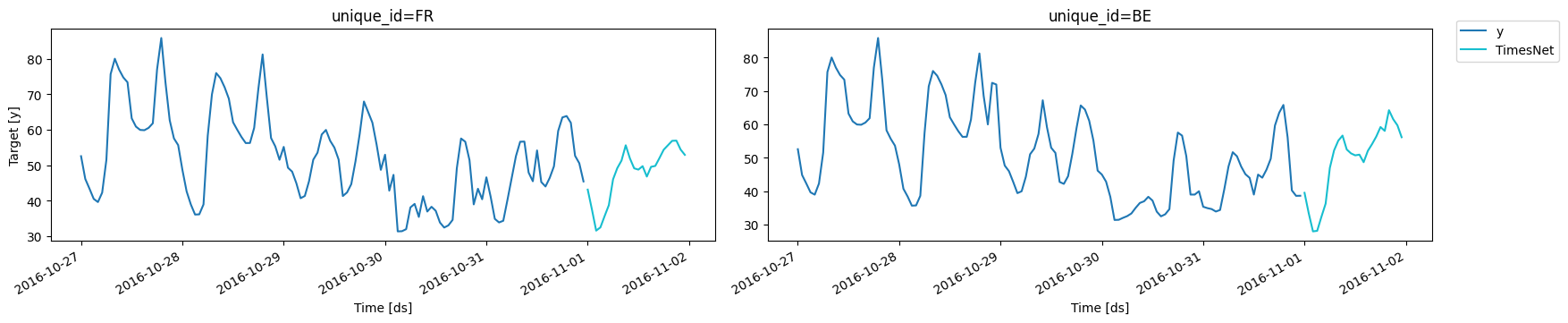
Finally, use the `predict` method to forecast the day-ahead prices. The
`Neuralforecast` class handles the inverse normalization, forecasts are
returned in the original scale.
```python theme={null}
Y_hat_df = nf.predict(futr_df=futr_df)
Y_hat_df.head()
```
```text theme={null}
Predicting: | …
```
| | unique\_id | ds | TimesNet |
| - | ---------- | ------------------- | --------- |
| 0 | BE | 2016-11-01 00:00:00 | 39.523182 |
| 1 | BE | 2016-11-01 01:00:00 | 33.386608 |
| 2 | BE | 2016-11-01 02:00:00 | 27.978468 |
| 3 | BE | 2016-11-01 03:00:00 | 28.143955 |
| 4 | BE | 2016-11-01 04:00:00 | 32.332230 |
```python theme={null}
from utilsforecast.plotting import plot_series
```
```python theme={null}
plot_series(df, Y_hat_df, max_insample_length=24*5)
```
## 1. Install `Neuralforecast`
```python theme={null}
%%capture
!pip install neuralforecast
!pip install hyperopt
```
## 2. Load Data
The `df` dataframe contains the target and exogenous variables past
information to train the model. The `unique_id` column identifies the
markets, `ds` contains the datestamps, and `y` the electricity price.
For future variables, we include a forecast of how much electricity will
be produced (`gen_forecast`), and day of week (`week_day`). Both the
electricity system demand and offer impact the price significantly,
including these variables to the model greatly improve performance, as
we demonstrate in Olivares et al. (2022).
The `futr_df` dataframe includes the information of the future exogenous
variables for the period we want to forecast (in this case, 24 hours
after the end of the train dataset `df`).
```python theme={null}
import pandas as pd
import matplotlib.pyplot as plt
```
```python theme={null}
df = pd.read_csv(
'https://datasets-nixtla.s3.amazonaws.com/EPF_FR_BE.csv',
parse_dates=['ds'],
)
futr_df = pd.read_csv(
'https://datasets-nixtla.s3.amazonaws.com/EPF_FR_BE_futr.csv',
parse_dates=['ds'],
)
df.head()
```
| | unique\_id | ds | y | gen\_forecast | system\_load | week\_day |
| - | ---------- | ------------------- | ----- | ------------- | ------------ | --------- |
| 0 | FR | 2015-01-01 00:00:00 | 53.48 | 76905.0 | 74812.0 | 3 |
| 1 | FR | 2015-01-01 01:00:00 | 51.93 | 75492.0 | 71469.0 | 3 |
| 2 | FR | 2015-01-01 02:00:00 | 48.76 | 74394.0 | 69642.0 | 3 |
| 3 | FR | 2015-01-01 03:00:00 | 42.27 | 72639.0 | 66704.0 | 3 |
| 4 | FR | 2015-01-01 04:00:00 | 38.41 | 69347.0 | 65051.0 | 3 |
We can see that `y` and the exogenous variables are on largely different
scales. Next, we show two methods to scale the data.
## 3. Time Series Scaling with `Neuralforecast` class
One of the most widely used approches for scaling time series is to
treat it as a pre-processing step, where each time series and temporal
exogenous variables are scaled based on their entire information in the
train set. Models are then trained on the scaled data.
To simplify pipelines, we added a scaling functionality to the
`Neuralforecast` class. Each time series will be scaled before training
the model with either `fit` or `cross_validation`, and scaling
statistics are stored. The class then uses the stored statistics to
scale the forecasts back to the original scale before returning the
forecasts.
### 3.a. Instantiate model and `Neuralforecast` class
In this example we will use the `TimesNet` model, recently proposed in
[Wu, Haixu, et al. (2022)](https://arxiv.org/abs/2210.02186). First
instantiate the model with the desired parameters.
```python theme={null}
import logging
from neuralforecast.models import TimesNet
from neuralforecast.core import NeuralForecast
```
```python theme={null}
logging.getLogger("pytorch_lightning").setLevel(logging.WARNING)
```
```python theme={null}
horizon = 24 # day-ahead daily forecast
model = TimesNet(h = horizon, # Horizon
input_size = 5*horizon, # Length of input window
max_steps = 100, # Training iterations
top_k = 3, # Number of periods (for FFT).
num_kernels = 3, # Number of kernels for Inception module
batch_size = 2, # Number of time series per batch
windows_batch_size = 32, # Number of windows per batch
learning_rate = 0.001, # Learning rate
futr_exog_list = ['gen_forecast', 'week_day'], # Future exogenous variables
scaler_type = None) # We use the Core scaling method
```
```text theme={null}
Seed set to 1
```
Fit the model by instantiating a `NeuralForecast` object and using the
`fit` method. The `local_scaler_type` parameter is used to specify the
type of scaling to be used. In this case, we will use `standard`, which
scales the data to have zero mean and unit variance.Other supported
scalers are `minmax`, `robust`, `robust-iqr`, `minmax`, and `boxcox`.
```python theme={null}
nf = NeuralForecast(models=[model], freq='h', local_scaler_type='standard')
nf.fit(df=df)
```
```text theme={null}
Sanity Checking: | …
```
```text theme={null}
Training: | …
```
```text theme={null}
Validation: | …
```
### 3.b Forecast and plots
Finally, use the `predict` method to forecast the day-ahead prices. The
`Neuralforecast` class handles the inverse normalization, forecasts are
returned in the original scale.
```python theme={null}
Y_hat_df = nf.predict(futr_df=futr_df)
Y_hat_df.head()
```
```text theme={null}
Predicting: | …
```
| | unique\_id | ds | TimesNet |
| - | ---------- | ------------------- | --------- |
| 0 | BE | 2016-11-01 00:00:00 | 39.523182 |
| 1 | BE | 2016-11-01 01:00:00 | 33.386608 |
| 2 | BE | 2016-11-01 02:00:00 | 27.978468 |
| 3 | BE | 2016-11-01 03:00:00 | 28.143955 |
| 4 | BE | 2016-11-01 04:00:00 | 32.332230 |
```python theme={null}
from utilsforecast.plotting import plot_series
```
```python theme={null}
plot_series(df, Y_hat_df, max_insample_length=24*5)
```
 > **Important**
>
> The inverse scaling is performed by the `Neuralforecast` class before
> returning the final forecasts. Therefore, the hyperparmater selection
> with `Auto` models and validation loss for early stopping or model
> selection are performed on the scaled data. Different types of scaling
> with the `Neuralforecast` class can’t be automatically compared with
> `Auto` models.
## 4. Temporal Window normalization during training
Temporal normalization scales each instance of the batch separately at
the window level. It is performed at each training iteration for each
window of the batch, for both target variable and temporal exogenous
covariates. For more details, see [Olivares et
al. (2023)](https://arxiv.org/abs/2305.07089) and
[https://nixtlaverse.nixtla.io/neuralforecast/common.scalers.html](https://nixtlaverse.nixtla.io/neuralforecast/common.scalers.html).
### 4.a. Instantiate model and `Neuralforecast` class
Temporal normalization is specified by the `scaler_type` argument.
Currently, it is only supported for Windows-based models (`NHITS`,
`NBEATS`, `MLP`, `TimesNet`, and all Transformers). In this example, we
use the `TimesNet` model and `robust` scaler, recently proposed by Wu,
Haixu, et al. (2022). First instantiate the model with the desired
parameters.
Visit [https://nixtlaverse.nixtla.io/neuralforecast/common.scalers.html](https://nixtlaverse.nixtla.io/neuralforecast/common.scalers.html)
for a complete list of supported scalers.
```python theme={null}
horizon = 24 # day-ahead daily forecast
model = TimesNet(h = horizon, # Horizon
input_size = 5*horizon, # Length of input window
max_steps = 100, # Training iterations
top_k = 3, # Number of periods (for FFT).
num_kernels = 3, # Number of kernels for Inception module
batch_size = 2, # Number of time series per batch
windows_batch_size = 32, # Number of windows per batch
learning_rate = 0.001, # Learning rate
futr_exog_list = ['gen_forecast','week_day'], # Future exogenous variables
scaler_type = 'robust') # Robust scaling
```
```text theme={null}
Seed set to 1
```
Fit the model by instantiating a `NeuralForecast` object and using the
`fit` method. Note that `local_scaler_type` has `None` as default to
avoid scaling the data before training.
```python theme={null}
nf = NeuralForecast(models=[model], freq='h')
nf.fit(df=df)
```
```text theme={null}
Sanity Checking: | …
```
```text theme={null}
Training: | …
```
```text theme={null}
Validation: | …
```
### 4.b Forecast and plots
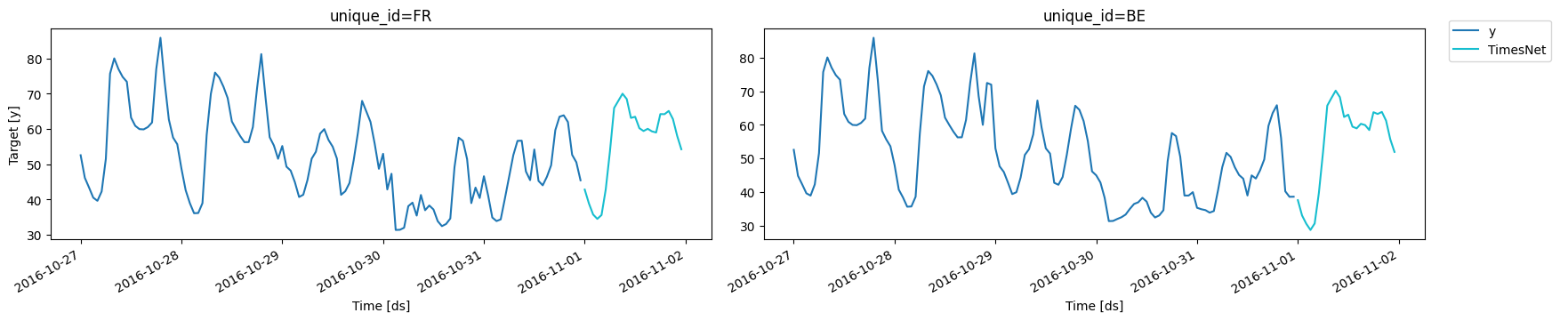
Finally, use the `predict` method to forecast the day-ahead prices. The
forecasts are returned in the original scale.
```python theme={null}
Y_hat_df = nf.predict(futr_df=futr_df)
Y_hat_df.head()
```
```text theme={null}
Predicting: | …
```
| | unique\_id | ds | TimesNet |
| - | ---------- | ------------------- | --------- |
| 0 | BE | 2016-11-01 00:00:00 | 37.624653 |
| 1 | BE | 2016-11-01 01:00:00 | 33.069824 |
| 2 | BE | 2016-11-01 02:00:00 | 30.623751 |
| 3 | BE | 2016-11-01 03:00:00 | 28.773439 |
| 4 | BE | 2016-11-01 04:00:00 | 30.689444 |
```python theme={null}
plot_series(df, Y_hat_df, max_insample_length=24*5)
```
> **Important**
>
> The inverse scaling is performed by the `Neuralforecast` class before
> returning the final forecasts. Therefore, the hyperparmater selection
> with `Auto` models and validation loss for early stopping or model
> selection are performed on the scaled data. Different types of scaling
> with the `Neuralforecast` class can’t be automatically compared with
> `Auto` models.
## 4. Temporal Window normalization during training
Temporal normalization scales each instance of the batch separately at
the window level. It is performed at each training iteration for each
window of the batch, for both target variable and temporal exogenous
covariates. For more details, see [Olivares et
al. (2023)](https://arxiv.org/abs/2305.07089) and
[https://nixtlaverse.nixtla.io/neuralforecast/common.scalers.html](https://nixtlaverse.nixtla.io/neuralforecast/common.scalers.html).
### 4.a. Instantiate model and `Neuralforecast` class
Temporal normalization is specified by the `scaler_type` argument.
Currently, it is only supported for Windows-based models (`NHITS`,
`NBEATS`, `MLP`, `TimesNet`, and all Transformers). In this example, we
use the `TimesNet` model and `robust` scaler, recently proposed by Wu,
Haixu, et al. (2022). First instantiate the model with the desired
parameters.
Visit [https://nixtlaverse.nixtla.io/neuralforecast/common.scalers.html](https://nixtlaverse.nixtla.io/neuralforecast/common.scalers.html)
for a complete list of supported scalers.
```python theme={null}
horizon = 24 # day-ahead daily forecast
model = TimesNet(h = horizon, # Horizon
input_size = 5*horizon, # Length of input window
max_steps = 100, # Training iterations
top_k = 3, # Number of periods (for FFT).
num_kernels = 3, # Number of kernels for Inception module
batch_size = 2, # Number of time series per batch
windows_batch_size = 32, # Number of windows per batch
learning_rate = 0.001, # Learning rate
futr_exog_list = ['gen_forecast','week_day'], # Future exogenous variables
scaler_type = 'robust') # Robust scaling
```
```text theme={null}
Seed set to 1
```
Fit the model by instantiating a `NeuralForecast` object and using the
`fit` method. Note that `local_scaler_type` has `None` as default to
avoid scaling the data before training.
```python theme={null}
nf = NeuralForecast(models=[model], freq='h')
nf.fit(df=df)
```
```text theme={null}
Sanity Checking: | …
```
```text theme={null}
Training: | …
```
```text theme={null}
Validation: | …
```
### 4.b Forecast and plots
Finally, use the `predict` method to forecast the day-ahead prices. The
forecasts are returned in the original scale.
```python theme={null}
Y_hat_df = nf.predict(futr_df=futr_df)
Y_hat_df.head()
```
```text theme={null}
Predicting: | …
```
| | unique\_id | ds | TimesNet |
| - | ---------- | ------------------- | --------- |
| 0 | BE | 2016-11-01 00:00:00 | 37.624653 |
| 1 | BE | 2016-11-01 01:00:00 | 33.069824 |
| 2 | BE | 2016-11-01 02:00:00 | 30.623751 |
| 3 | BE | 2016-11-01 03:00:00 | 28.773439 |
| 4 | BE | 2016-11-01 04:00:00 | 30.689444 |
```python theme={null}
plot_series(df, Y_hat_df, max_insample_length=24*5)
```
 > **Important**
>
> For most applications, models with temporal normalization (section 4)
> produced more accurate forecasts than time series scaling (section 3).
> However, with temporal normalization models lose the information of
> the relative level between different windows. In some cases this
> global information within time series is crucial, for instance when an
> exogenous variables contains the dosage of a medication. In these
> cases, time series scaling (section 3) is preferred.
## References
* [Kin G. Olivares, David Luo, Cristian Challu, Stefania La Vattiata,
Max Mergenthaler, Artur Dubrawski (2023). “HINT: Hierarchical
Mixture Networks For Coherent Probabilistic Forecasting”.
International Conference on Machine Learning (ICML). Workshop on
Structured Probabilistic Inference & Generative Modeling. Available
at
https://arxiv.org/abs/2305.07089.](https://arxiv.org/abs/2305.07089)
* [Wu, Haixu, Tengge Hu, Yong Liu, Hang Zhou, Jianmin Wang, and
Mingsheng Long. “Timesnet: Temporal 2d-variation modeling for
general time series analysis.”, ICLR
2023](https://openreview.net/forum?id=ju_Uqw384Oq)
> **Important**
>
> For most applications, models with temporal normalization (section 4)
> produced more accurate forecasts than time series scaling (section 3).
> However, with temporal normalization models lose the information of
> the relative level between different windows. In some cases this
> global information within time series is crucial, for instance when an
> exogenous variables contains the dosage of a medication. In these
> cases, time series scaling (section 3) is preferred.
## References
* [Kin G. Olivares, David Luo, Cristian Challu, Stefania La Vattiata,
Max Mergenthaler, Artur Dubrawski (2023). “HINT: Hierarchical
Mixture Networks For Coherent Probabilistic Forecasting”.
International Conference on Machine Learning (ICML). Workshop on
Structured Probabilistic Inference & Generative Modeling. Available
at
https://arxiv.org/abs/2305.07089.](https://arxiv.org/abs/2305.07089)
* [Wu, Haixu, Tengge Hu, Yong Liu, Hang Zhou, Jianmin Wang, and
Mingsheng Long. “Timesnet: Temporal 2d-variation modeling for
general time series analysis.”, ICLR
2023](https://openreview.net/forum?id=ju_Uqw384Oq)