> ## Documentation Index
> Fetch the complete documentation index at: https://nixtlaverse.nixtla.io/llms.txt
> Use this file to discover all available pages before exploring further.
# Exogenous Variables
Exogenous variables can provide additional information to greatly
improve forecasting accuracy. Some examples include price or future
promotions variables for demand forecasting, and weather data for
electricity load forecast. In this notebook we show an example on how to
add different types of exogenous variables to NeuralForecast models for
making day-ahead hourly electricity price forecasts (EPF) for France and
Belgium markets.
All NeuralForecast models are capable of incorporating exogenous
variables to model the following conditional predictive distribution:
$\mathbb{P}(\mathbf{y}_{t+1:t+H} \;|\; \mathbf{y}_{[:t]},\; \mathbf{x}^{(h)}_{[:t]},\; \mathbf{x}^{(f)}_{[:t+H]},\; \mathbf{x}^{(s)} )$
where the regressors are static exogenous $\mathbf{x}^{(s)}$, historic
exogenous $\mathbf{x}^{(h)}_{[:t]}$, exogenous available at the time of
the prediction $\mathbf{x}^{(f)}_{[:t+H]}$ and autoregressive features
$\mathbf{y}_{[:t]}$. Depending on the [train
loss](../../losses.pytorch.html), the model outputs can be point
forecasts (location estimators) or uncertainty intervals (quantiles).
We will show you how to include exogenous variables in the data, specify
variables to a model, and produce forecasts using future exogenous
variables.
> **Important**
>
> This Guide assumes basic knowledge on the NeuralForecast library. For
> a minimal example visit the [Getting
> Started](../getting-started/quickstart.html) guide.
You can run these experiments using GPU with Google Colab.
 ## 1. Libraries
```python theme={null}
%%capture
!pip install neuralforecast
```
## 2. Load data
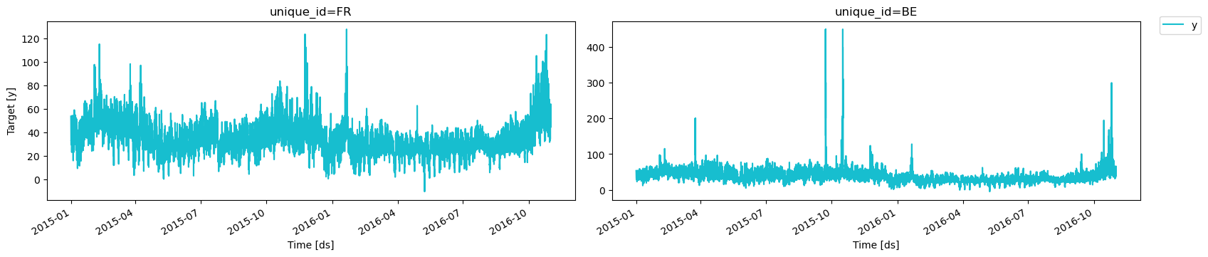
The `df` dataframe contains the target and exogenous variables past
information to train the model. The `unique_id` column identifies the
markets, `ds` contains the datestamps, and `y` the electricity price.
Include both historic and future temporal variables as columns. In this
example, we are adding the system load (`system_load`) as historic data.
For future variables, we include a forecast of how much electricity will
be produced (`gen_forecast`) and day of week (`week_day`). Both the
electricity system demand and offer impact the price significantly,
including these variables to the model greatly improve performance, as
we demonstrate in Olivares et al. (2022).
The distinction between historic and future variables will be made later
as parameters of the model.
```python theme={null}
import pandas as pd
from utilsforecast.plotting import plot_series
```
```python theme={null}
df = pd.read_csv(
'https://datasets-nixtla.s3.amazonaws.com/EPF_FR_BE.csv',
parse_dates=['ds'],
)
df.head()
```
| | unique\_id | ds | y | gen\_forecast | system\_load | week\_day |
| - | ---------- | ------------------- | ----- | ------------- | ------------ | --------- |
| 0 | FR | 2015-01-01 00:00:00 | 53.48 | 76905.0 | 74812.0 | 3 |
| 1 | FR | 2015-01-01 01:00:00 | 51.93 | 75492.0 | 71469.0 | 3 |
| 2 | FR | 2015-01-01 02:00:00 | 48.76 | 74394.0 | 69642.0 | 3 |
| 3 | FR | 2015-01-01 03:00:00 | 42.27 | 72639.0 | 66704.0 | 3 |
| 4 | FR | 2015-01-01 04:00:00 | 38.41 | 69347.0 | 65051.0 | 3 |
> **Tip**
>
> Calendar variables such as day of week, month, and year are very
> useful to capture long seasonalities.
```python theme={null}
plot_series(df)
```
## 1. Libraries
```python theme={null}
%%capture
!pip install neuralforecast
```
## 2. Load data
The `df` dataframe contains the target and exogenous variables past
information to train the model. The `unique_id` column identifies the
markets, `ds` contains the datestamps, and `y` the electricity price.
Include both historic and future temporal variables as columns. In this
example, we are adding the system load (`system_load`) as historic data.
For future variables, we include a forecast of how much electricity will
be produced (`gen_forecast`) and day of week (`week_day`). Both the
electricity system demand and offer impact the price significantly,
including these variables to the model greatly improve performance, as
we demonstrate in Olivares et al. (2022).
The distinction between historic and future variables will be made later
as parameters of the model.
```python theme={null}
import pandas as pd
from utilsforecast.plotting import plot_series
```
```python theme={null}
df = pd.read_csv(
'https://datasets-nixtla.s3.amazonaws.com/EPF_FR_BE.csv',
parse_dates=['ds'],
)
df.head()
```
| | unique\_id | ds | y | gen\_forecast | system\_load | week\_day |
| - | ---------- | ------------------- | ----- | ------------- | ------------ | --------- |
| 0 | FR | 2015-01-01 00:00:00 | 53.48 | 76905.0 | 74812.0 | 3 |
| 1 | FR | 2015-01-01 01:00:00 | 51.93 | 75492.0 | 71469.0 | 3 |
| 2 | FR | 2015-01-01 02:00:00 | 48.76 | 74394.0 | 69642.0 | 3 |
| 3 | FR | 2015-01-01 03:00:00 | 42.27 | 72639.0 | 66704.0 | 3 |
| 4 | FR | 2015-01-01 04:00:00 | 38.41 | 69347.0 | 65051.0 | 3 |
> **Tip**
>
> Calendar variables such as day of week, month, and year are very
> useful to capture long seasonalities.
```python theme={null}
plot_series(df)
```
 Add the static variables in a separate `static_df` dataframe. In this
example, we are using one-hot encoding of the electricity market. The
`static_df` must include one observation (row) for each `unique_id` of
the `df` dataframe, with the different statics variables as columns.
```python theme={null}
static_df = pd.read_csv('https://datasets-nixtla.s3.amazonaws.com/EPF_FR_BE_static.csv')
static_df.head()
```
| | unique\_id | market\_0 | market\_1 |
| - | ---------- | --------- | --------- |
| 0 | FR | 1 | 0 |
| 1 | BR | 0 | 1 |
## 3. Training with exogenous variables
We distinguish the exogenous variables by whether they reflect static or
time-dependent aspects of the modeled data.
* **Static exogenous variables**: The static exogenous variables carry
time-invariant information for each time series. When the model is
built with global parameters to forecast multiple time series, these
variables allow sharing information within groups of time series
with similar static variable levels. Examples of static variables
include designators such as identifiers of regions, groups of
products, etc.
* **Historic exogenous variables**: This time-dependent exogenous
variable is restricted to past observed values. Its predictive power
depends on Granger-causality, as its past values can provide
significant information about future values of the target variable
$\mathbf{y}$.
* **Future exogenous variables**: In contrast with historic exogenous
variables, future values are available at the time of the
prediction. Examples include calendar variables, weather forecasts,
and known events that can cause large spikes and dips such as
scheduled promotions.
To add exogenous variables to the model, first specify the name of each
variable from the previous dataframes to the corresponding model
hyperparameter during initialization: `futr_exog_list`,
`hist_exog_list`, and `stat_exog_list`. We also set `horizon` as 24 to
produce the next day hourly forecasts, and set `input_size` to use the
last 5 days of data as input.
```python theme={null}
import logging
from neuralforecast.auto import NHITS, BiTCN
from neuralforecast.core import NeuralForecast
```
```python theme={null}
logging.getLogger("pytorch_lightning").setLevel(logging.WARNING)
```
```python theme={null}
horizon = 24 # day-ahead daily forecast
models = [NHITS(h = horizon,
max_steps=100,
input_size = 5*horizon,
futr_exog_list = ['gen_forecast', 'week_day'], # <- Future exogenous variables
hist_exog_list = ['system_load'], # <- Historical exogenous variables
stat_exog_list = ['market_0', 'market_1'], # <- Static exogenous variables
scaler_type = 'robust'),
BiTCN(h = horizon,
input_size = 5*horizon,
max_steps=100,
futr_exog_list = ['gen_forecast', 'week_day'], # <- Future exogenous variables
hist_exog_list = ['system_load'], # <- Historical exogenous variables
stat_exog_list = ['market_0', 'market_1'], # <- Static exogenous variables
scaler_type = 'robust',
),
]
```
```text theme={null}
Seed set to 1
Seed set to 1
```
> **Tip**
>
> When including exogenous variables always use a scaler by setting the
> `scaler_type` hyperparameter. The scaler will scale all the temporal
> features: the target variable `y`, historic and future variables.
> **Important**
>
> Make sure future and historic variables are correctly placed. Defining
> historic variables as future variables will lead to data leakage.
Next, pass the datasets to the `df` and `static_df` inputs of the `fit`
method.
> **Tip**
>
> You can scale static variables using the `local_static_scaler_type`
> parameter when initializing a `NeuralForecast` instance.
```python theme={null}
nf = NeuralForecast(models=models, freq='h')
nf.fit(df=df, static_df=static_df)
```
## 4. Forecasting with exogenous variables
Before predicting the prices, we need to gather the future exogenous
variables for the day we want to forecast. Define a new dataframe
(`futr_df`) with the `unique_id`, `ds`, and future exogenous variables.
There is no need to add the target variable `y` and historic variables
as they won’t be used by the model.
```python theme={null}
futr_df = pd.read_csv(
'https://datasets-nixtla.s3.amazonaws.com/EPF_FR_BE_futr.csv',
parse_dates=['ds'],
)
futr_df.head()
```
| | unique\_id | ds | gen\_forecast | week\_day |
| - | ---------- | ------------------- | ------------- | --------- |
| 0 | FR | 2016-11-01 00:00:00 | 49118.0 | 1 |
| 1 | FR | 2016-11-01 01:00:00 | 47890.0 | 1 |
| 2 | FR | 2016-11-01 02:00:00 | 47158.0 | 1 |
| 3 | FR | 2016-11-01 03:00:00 | 45991.0 | 1 |
| 4 | FR | 2016-11-01 04:00:00 | 45378.0 | 1 |
> **Important**
>
> Make sure `futr_df` has informations for the entire forecast horizon.
> In this example, we are forecasting 24 hours ahead, so `futr_df` must
> have 24 rows for each time series.
Finally, use the `predict` method to forecast the day-ahead prices.
```python theme={null}
Y_hat_df = nf.predict(futr_df=futr_df)
Y_hat_df.head()
```
```text theme={null}
Predicting: | | 0/? [00:00
In summary, to add exogenous variables to a model make sure to follow
the next steps:
1. Add temporal exogenous variables as columns to the main dataframe
(`df`).
2. Add static exogenous variables with the `static_df` dataframe.
3. Specify the name for each variable in the corresponding model
hyperparameter.
4. If the model uses future exogenous variables, pass the future
dataframe (`futr_df`) to the `predict` method.
## References
* [Kin G. Olivares, Cristian Challu, Grzegorz Marcjasz, Rafał Weron,
Artur Dubrawski, Neural basis expansion analysis with exogenous
variables: Forecasting electricity prices with NBEATSx,
International Journal of
Forecasting](https://www.sciencedirect.com/science/article/pii/S0169207022000413)
* [Cristian Challu, Kin G. Olivares, Boris N. Oreshkin, Federico
Garza, Max Mergenthaler-Canseco, Artur Dubrawski (2021). NHITS:
Neural Hierarchical Interpolation for Time Series Forecasting.
Accepted at AAAI 2023.](https://arxiv.org/abs/2201.12886)
Add the static variables in a separate `static_df` dataframe. In this
example, we are using one-hot encoding of the electricity market. The
`static_df` must include one observation (row) for each `unique_id` of
the `df` dataframe, with the different statics variables as columns.
```python theme={null}
static_df = pd.read_csv('https://datasets-nixtla.s3.amazonaws.com/EPF_FR_BE_static.csv')
static_df.head()
```
| | unique\_id | market\_0 | market\_1 |
| - | ---------- | --------- | --------- |
| 0 | FR | 1 | 0 |
| 1 | BR | 0 | 1 |
## 3. Training with exogenous variables
We distinguish the exogenous variables by whether they reflect static or
time-dependent aspects of the modeled data.
* **Static exogenous variables**: The static exogenous variables carry
time-invariant information for each time series. When the model is
built with global parameters to forecast multiple time series, these
variables allow sharing information within groups of time series
with similar static variable levels. Examples of static variables
include designators such as identifiers of regions, groups of
products, etc.
* **Historic exogenous variables**: This time-dependent exogenous
variable is restricted to past observed values. Its predictive power
depends on Granger-causality, as its past values can provide
significant information about future values of the target variable
$\mathbf{y}$.
* **Future exogenous variables**: In contrast with historic exogenous
variables, future values are available at the time of the
prediction. Examples include calendar variables, weather forecasts,
and known events that can cause large spikes and dips such as
scheduled promotions.
To add exogenous variables to the model, first specify the name of each
variable from the previous dataframes to the corresponding model
hyperparameter during initialization: `futr_exog_list`,
`hist_exog_list`, and `stat_exog_list`. We also set `horizon` as 24 to
produce the next day hourly forecasts, and set `input_size` to use the
last 5 days of data as input.
```python theme={null}
import logging
from neuralforecast.auto import NHITS, BiTCN
from neuralforecast.core import NeuralForecast
```
```python theme={null}
logging.getLogger("pytorch_lightning").setLevel(logging.WARNING)
```
```python theme={null}
horizon = 24 # day-ahead daily forecast
models = [NHITS(h = horizon,
max_steps=100,
input_size = 5*horizon,
futr_exog_list = ['gen_forecast', 'week_day'], # <- Future exogenous variables
hist_exog_list = ['system_load'], # <- Historical exogenous variables
stat_exog_list = ['market_0', 'market_1'], # <- Static exogenous variables
scaler_type = 'robust'),
BiTCN(h = horizon,
input_size = 5*horizon,
max_steps=100,
futr_exog_list = ['gen_forecast', 'week_day'], # <- Future exogenous variables
hist_exog_list = ['system_load'], # <- Historical exogenous variables
stat_exog_list = ['market_0', 'market_1'], # <- Static exogenous variables
scaler_type = 'robust',
),
]
```
```text theme={null}
Seed set to 1
Seed set to 1
```
> **Tip**
>
> When including exogenous variables always use a scaler by setting the
> `scaler_type` hyperparameter. The scaler will scale all the temporal
> features: the target variable `y`, historic and future variables.
> **Important**
>
> Make sure future and historic variables are correctly placed. Defining
> historic variables as future variables will lead to data leakage.
Next, pass the datasets to the `df` and `static_df` inputs of the `fit`
method.
> **Tip**
>
> You can scale static variables using the `local_static_scaler_type`
> parameter when initializing a `NeuralForecast` instance.
```python theme={null}
nf = NeuralForecast(models=models, freq='h')
nf.fit(df=df, static_df=static_df)
```
## 4. Forecasting with exogenous variables
Before predicting the prices, we need to gather the future exogenous
variables for the day we want to forecast. Define a new dataframe
(`futr_df`) with the `unique_id`, `ds`, and future exogenous variables.
There is no need to add the target variable `y` and historic variables
as they won’t be used by the model.
```python theme={null}
futr_df = pd.read_csv(
'https://datasets-nixtla.s3.amazonaws.com/EPF_FR_BE_futr.csv',
parse_dates=['ds'],
)
futr_df.head()
```
| | unique\_id | ds | gen\_forecast | week\_day |
| - | ---------- | ------------------- | ------------- | --------- |
| 0 | FR | 2016-11-01 00:00:00 | 49118.0 | 1 |
| 1 | FR | 2016-11-01 01:00:00 | 47890.0 | 1 |
| 2 | FR | 2016-11-01 02:00:00 | 47158.0 | 1 |
| 3 | FR | 2016-11-01 03:00:00 | 45991.0 | 1 |
| 4 | FR | 2016-11-01 04:00:00 | 45378.0 | 1 |
> **Important**
>
> Make sure `futr_df` has informations for the entire forecast horizon.
> In this example, we are forecasting 24 hours ahead, so `futr_df` must
> have 24 rows for each time series.
Finally, use the `predict` method to forecast the day-ahead prices.
```python theme={null}
Y_hat_df = nf.predict(futr_df=futr_df)
Y_hat_df.head()
```
```text theme={null}
Predicting: | | 0/? [00:00
In summary, to add exogenous variables to a model make sure to follow
the next steps:
1. Add temporal exogenous variables as columns to the main dataframe
(`df`).
2. Add static exogenous variables with the `static_df` dataframe.
3. Specify the name for each variable in the corresponding model
hyperparameter.
4. If the model uses future exogenous variables, pass the future
dataframe (`futr_df`) to the `predict` method.
## References
* [Kin G. Olivares, Cristian Challu, Grzegorz Marcjasz, Rafał Weron,
Artur Dubrawski, Neural basis expansion analysis with exogenous
variables: Forecasting electricity prices with NBEATSx,
International Journal of
Forecasting](https://www.sciencedirect.com/science/article/pii/S0169207022000413)
* [Cristian Challu, Kin G. Olivares, Boris N. Oreshkin, Federico
Garza, Max Mergenthaler-Canseco, Artur Dubrawski (2021). NHITS:
Neural Hierarchical Interpolation for Time Series Forecasting.
Accepted at AAAI 2023.](https://arxiv.org/abs/2201.12886)