> ## Documentation Index
> Fetch the complete documentation index at: https://nixtlaverse.nixtla.io/llms.txt
> Use this file to discover all available pages before exploring further.
# Transfer Conformal Prediction Intervals
This tutorial evaluates the **conformal prediction transfer methods**
available in `mlforecast`. We train a model on one domain (M4 Monthly
**Macro** series) and then generate calibrated prediction intervals for
a different domain (M4 Monthly **Finance** series) — without retraining
the model.
## Why transfer?
Standard conformal prediction intervals are calibrated on the same
distribution as training data. When you apply a pretrained model to
**new, unseen series** from a potentially different domain, the source
conformity scores may be miscalibrated for the target domain. Transfer
conformal methods attempt to correct for this shift using different
strategies:
| Method | Strategy | Needs CV on target? |
| ------------------------ | --------------------------------------------------------------------- | ------------------- |
| `recalibrate` | Re-run cross-validation on target data | Yes |
| `scale_aligned` | Rescale source errors by target/source scale ratio (from *y* history) | No |
| `error_scaled` | Rescale source errors by target/source prediction error ratio | Yes |
| `weighted_conformal` | Reweight source errors via density-ratio estimation (covariate shift) | No |
| `scale_aligned_weighted` | Combine scale alignment with density-ratio weighting | No |
We evaluate each method’s **empirical coverage** — the fraction of test
observations that fall inside the predicted interval — and compare it to
the nominal level.
## Setup
```python theme={null}
import warnings
warnings.filterwarnings('ignore')
import lightgbm as lgb
import numpy as np
import pandas as pd
import matplotlib.pyplot as plt
from sklearn.preprocessing import FunctionTransformer
from mlforecast import MLForecast
from mlforecast.lag_transforms import (
ExpandingMean,
ExponentiallyWeightedMean,
RollingMean,
RollingStd,
SeasonalRollingMean,
)
from mlforecast.target_transforms import Differences, GlobalSklearnTransformer
from mlforecast.utils import PredictionIntervals
```
## Load M4 Monthly Data
The M4 Monthly dataset contains 48,000 monthly time series across 6
categories. We use it to create a cross-domain transfer scenario:
* **Source domain**: `Macro` category — macroeconomic time series
* **Target domain**: `Finance` category — financial time series
The forecast horizon for M4 Monthly is **h = 18** months.
```python theme={null}
HORIZON = 18
DATA_DIR = '../../../data'
def read_and_melt(file):
df = pd.read_csv(file)
df.columns = ['unique_id'] + list(range(1, df.shape[1]))
df = pd.melt(df, id_vars=['unique_id'], var_name='ds', value_name='y')
df = df.dropna()
df['ds'] = df['ds'].astype(int)
return df
# Load train/test splits (M4 stores them separately)
m4_train = read_and_melt(f'{DATA_DIR}/m4/datasets/Monthly-train.csv')
m4_test = read_and_melt(f'{DATA_DIR}/m4/datasets/Monthly-test.csv')
# Adjust test ds so it continues from where train ends
last_train_ds = m4_train.groupby('unique_id')['ds'].max().reset_index()
last_train_ds.columns = ['unique_id', 'last_ds']
m4_test = m4_test.merge(last_train_ds, on='unique_id')
m4_test['ds'] = m4_test['ds'] + m4_test['last_ds']
m4_test = m4_test.drop(columns='last_ds')
print(f"Train: {m4_train.shape}, Test: {m4_test.shape}")
print(f"Training series count: {m4_train['unique_id'].nunique()}")
print(f"Test periods per series: {m4_test.groupby('unique_id')['ds'].count().unique().tolist()}")
```
```text theme={null}
Train: (10382411, 3), Test: (864000, 3)
Training series count: 48000
Test periods per series: [18]
```
```python theme={null}
# Load category labels from M4 info
m4_info = pd.read_csv(f'{DATA_DIR}/m4/datasets/M4-info.csv', usecols=['M4id', 'category'])
m4_info = m4_info[m4_info['M4id'].str.startswith('M')].rename(columns={'M4id': 'unique_id'})
print("M4 Monthly category counts:")
print(m4_info['category'].value_counts())
```
```text theme={null}
M4 Monthly category counts:
category
Finance 10987
Micro 10975
Industry 10017
Macro 10016
Demographic 5728
Other 277
Name: count, dtype: int64
```
## Create Source and Target Domains
```python theme={null}
rng = np.random.default_rng(42)
# Source domain: sample from Macro category
macro_ids = m4_info[m4_info['category'] == 'Macro']['unique_id'].values
source_ids = rng.choice(macro_ids, size=800, replace=False)
# Target domain: sample from Finance category (disjoint from source)
finance_ids = m4_info[m4_info['category'] == 'Finance']['unique_id'].values
target_ids = rng.choice(finance_ids, size=200, replace=False)
# Source: use all training data (no test split needed for fitting)
source_train = m4_train[m4_train['unique_id'].isin(source_ids)].copy()
# Target: training data goes into new_df; test data is our evaluation ground truth
target_train = m4_train[m4_train['unique_id'].isin(target_ids)].copy()
target_test = m4_test[m4_test['unique_id'].isin(target_ids)].copy()
print(f"Source domain: {source_train['unique_id'].nunique()} Macro series")
print(f" Train obs: {len(source_train):,}")
print(f" Length range: {source_train.groupby('unique_id')['ds'].count().agg(['min','max']).to_dict()}")
print()
print(f"Target domain: {target_train['unique_id'].nunique()} Finance series")
print(f" Train obs: {len(target_train):,}")
print(f" Test obs: {len(target_test):,} ({HORIZON} steps per series)")
```
```text theme={null}
Source domain: 800 Macro series
Train obs: 186,308
Length range: {'min': 62, 'max': 1230}
Target domain: 200 Finance series
Train obs: 38,794
Test obs: 3,600 (18 steps per series)
```
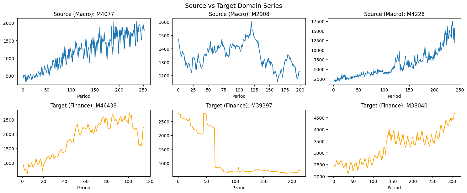
## Explore the Domains
Let’s visualize a few series from each domain to get a sense of the
distribution shift.
```python theme={null}
fig, axes = plt.subplots(2, 3, figsize=(15, 6))
sample_source = source_ids[:3]
sample_target = target_ids[:3]
for ax, uid in zip(axes[0], sample_source):
s = source_train[source_train['unique_id'] == uid]
ax.plot(s['ds'], s['y'])
ax.set_title(f'Source (Macro): {uid}')
ax.set_xlabel('Period')
for ax, uid in zip(axes[1], sample_target):
s = target_train[target_train['unique_id'] == uid]
ax.plot(s['ds'], s['y'], color='orange')
ax.set_title(f'Target (Finance): {uid}')
ax.set_xlabel('Period')
plt.tight_layout()
plt.suptitle('Source vs Target Domain Series', y=1.02, fontsize=14)
plt.show()
```
 ## Fit MLForecast on Source Domain
### Feature engineering for cross-domain transfer
Because the model is trained on one domain and applied to another, the
features must be **scale-invariant**. Tree models cannot extrapolate: if
a Finance series has level changes larger than anything seen in the
Macro training data, its predictions get clamped to the training range,
producing large, skewed errors that no conformal correction can fully
repair.
We therefore model **log-returns** instead of raw differences:
* `GlobalSklearnTransformer(FunctionTransformer(np.log1p, np.expm1))`
followed by `Differences([1])` — the model sees relative changes,
which live on a comparable scale in both domains. Back-transformed
intervals scale multiplicatively with each series’ level.
* Volatility and trend features (`RollingStd`,
`ExponentiallyWeightedMean`, `SeasonalRollingMean`) — these sharpen
the point forecasts and, importantly, give the density-ratio
estimator meaningful covariates: on the raw scale, lag features
mostly encode the scale difference between domains rather than the
dynamics.
### Prediction interval configuration
We fit on Macro series using `PredictionIntervals` with: -
`method='weighted_conformal_error'` — stores lag features in the
conformity score dataframe, enabling density-ratio estimation (DRE) for
the `weighted_conformal` and `scale_aligned_weighted` transfer
methods. - `scale_estimator='mad'` — stores per-series scale estimates
(MAD of first differences), enabling the `scale_aligned` and
`scale_aligned_weighted` transfer methods.
Using this single fit configuration unlocks **all five** transfer
methods.
```python theme={null}
mlf = MLForecast(
models=lgb.LGBMRegressor(n_estimators=100, verbosity=-1, random_state=0),
freq=1,
lags=[1, 2, 3, 4, 6, 12],
lag_transforms={
1: [
ExpandingMean(),
RollingMean(window_size=3),
RollingStd(window_size=12, min_samples=6),
ExponentiallyWeightedMean(alpha=0.3),
],
12: [SeasonalRollingMean(season_length=12, window_size=2, min_samples=1)],
},
target_transforms=[
GlobalSklearnTransformer(FunctionTransformer(func=np.log1p, inverse_func=np.expm1)),
Differences([1]),
],
num_threads=1,
)
mlf.fit(
source_train,
prediction_intervals=PredictionIntervals(
n_windows=2,
h=HORIZON,
method='weighted_conformal_error',
scale_estimator='mad',
),
)
```
```text theme={null}
MLForecast(models=[LGBMRegressor], freq=1, lag_features=['lag1', 'lag2', 'lag3', 'lag4', 'lag6', 'lag12', 'expanding_mean_lag1', 'rolling_mean_lag1_window_size3', 'rolling_std_lag1_window_size12_min_samples6', 'exponentially_weighted_mean_lag1_alpha0.3', 'seasonal_rolling_mean_lag12_season_length12_window_size2_min_samples1'], date_features=[], num_threads=1)
```
## Evaluate Transfer Methods
For each transfer method, we call `mlf.predict()` with: -
`new_df=target_train` — the target domain training history (Finance
series) - `level=[80, 90, 95]` — the requested coverage levels -
`transfer_conformal=method` — which transfer strategy to use
We then merge predictions with `target_test` and compute the **empirical
coverage** at each level.
```python theme={null}
LEVELS = [80, 90, 95]
MODEL = 'LGBMRegressor'
transfer_methods = [
'recalibrate',
'scale_aligned',
'error_scaled',
'weighted_conformal',
'scale_aligned_weighted',
]
coverage_results = {}
for method in transfer_methods:
print(f"Running '{method}'...", end=' ', flush=True)
preds = mlf.predict(
h=HORIZON,
level=LEVELS,
new_df=target_train,
transfer_conformal=method,
)
merged = target_test.merge(preds, on=['unique_id', 'ds'])
cov = {}
for lv in LEVELS:
lo_col = f'{MODEL}-lo-{lv}'
hi_col = f'{MODEL}-hi-{lv}'
covered = (merged['y'] >= merged[lo_col]) & (merged['y'] <= merged[hi_col])
cov[lv] = float(covered.mean())
coverage_results[method] = cov
print(f"done. Coverage: { {k: f'{v:.1%}' for k,v in cov.items()} }")
print("\nAll methods evaluated.")
```
```text theme={null}
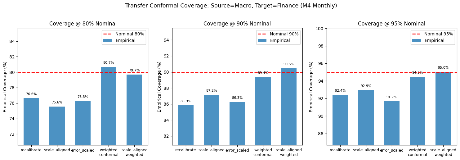
Running 'recalibrate'... done. Coverage: {80: '76.6%', 90: '85.9%', 95: '92.4%'}
Running 'scale_aligned'... done. Coverage: {80: '75.6%', 90: '87.2%', 95: '92.9%'}
Running 'error_scaled'... done. Coverage: {80: '76.3%', 90: '86.3%', 95: '91.7%'}
Running 'weighted_conformal'... done. Coverage: {80: '80.7%', 90: '89.4%', 95: '94.5%'}
Running 'scale_aligned_weighted'... done. Coverage: {80: '79.7%', 90: '90.5%', 95: '95.0%'}
All methods evaluated.
```
## Results: Nominal vs Empirical Coverage
A well-calibrated method should have empirical coverage close to
nominal. We show the results as a summary table and a bar chart.
```python theme={null}
# Build results dataframe
rows = []
for method, cov_dict in coverage_results.items():
for lv, empirical in cov_dict.items():
rows.append({
'Method': method,
'Nominal Level': f'{lv}%',
'Nominal': lv / 100,
'Empirical': empirical,
'Gap': empirical - lv / 100,
})
results_df = pd.DataFrame(rows)
# Pivot for display
pivot = results_df.pivot(index='Method', columns='Nominal Level', values='Empirical')
pivot = pivot[['80%', '90%', '95%']]
pivot.columns.name = 'Empirical Coverage @'
display_df = (pivot * 100).round(1).astype(str) + '%'
print("Empirical Coverage by Transfer Method (nominal levels: 80%, 90%, 95%)")
print("=" * 70)
print(display_df.to_string())
```
```text theme={null}
Empirical Coverage by Transfer Method (nominal levels: 80%, 90%, 95%)
======================================================================
Empirical Coverage @ 80% 90% 95%
Method
error_scaled 76.3% 86.3% 91.7%
recalibrate 76.6% 85.9% 92.4%
scale_aligned 75.6% 87.2% 92.9%
scale_aligned_weighted 79.7% 90.5% 95.0%
weighted_conformal 80.7% 89.4% 94.5%
```
```python theme={null}
# Bar chart: empirical vs nominal coverage
fig, axes = plt.subplots(1, 3, figsize=(15, 5), sharey=False)
method_labels = [
'recalibrate',
'scale_aligned',
'error_scaled',
'weighted\nconformal',
'scale_aligned\nweighted',
]
x = np.arange(len(transfer_methods))
for ax, lv in zip(axes, LEVELS):
empirical_vals = [coverage_results[m][lv] * 100 for m in transfer_methods]
bars = ax.bar(x, empirical_vals, width=0.6, alpha=0.8, label='Empirical')
ax.axhline(lv, color='red', linewidth=2, linestyle='--', label=f'Nominal {lv}%')
ax.set_xticks(x)
ax.set_xticklabels(method_labels, fontsize=9)
ax.set_title(f'Coverage @ {lv}% Nominal', fontsize=12)
ax.set_ylabel('Empirical Coverage (%)')
ax.legend()
# Add value labels on bars
for bar, val in zip(bars, empirical_vals):
ax.text(
bar.get_x() + bar.get_width() / 2,
bar.get_height() + 0.3,
f'{val:.1f}%',
ha='center', va='bottom', fontsize=8
)
y_min = min(min(empirical_vals), lv) - 5
y_max = max(max(empirical_vals), lv) + 5
ax.set_ylim(y_min, y_max)
plt.suptitle(
'Transfer Conformal Coverage: Source=Macro, Target=Finance (M4 Monthly)',
fontsize=13, y=1.02
)
plt.tight_layout()
plt.show()
```
## Fit MLForecast on Source Domain
### Feature engineering for cross-domain transfer
Because the model is trained on one domain and applied to another, the
features must be **scale-invariant**. Tree models cannot extrapolate: if
a Finance series has level changes larger than anything seen in the
Macro training data, its predictions get clamped to the training range,
producing large, skewed errors that no conformal correction can fully
repair.
We therefore model **log-returns** instead of raw differences:
* `GlobalSklearnTransformer(FunctionTransformer(np.log1p, np.expm1))`
followed by `Differences([1])` — the model sees relative changes,
which live on a comparable scale in both domains. Back-transformed
intervals scale multiplicatively with each series’ level.
* Volatility and trend features (`RollingStd`,
`ExponentiallyWeightedMean`, `SeasonalRollingMean`) — these sharpen
the point forecasts and, importantly, give the density-ratio
estimator meaningful covariates: on the raw scale, lag features
mostly encode the scale difference between domains rather than the
dynamics.
### Prediction interval configuration
We fit on Macro series using `PredictionIntervals` with: -
`method='weighted_conformal_error'` — stores lag features in the
conformity score dataframe, enabling density-ratio estimation (DRE) for
the `weighted_conformal` and `scale_aligned_weighted` transfer
methods. - `scale_estimator='mad'` — stores per-series scale estimates
(MAD of first differences), enabling the `scale_aligned` and
`scale_aligned_weighted` transfer methods.
Using this single fit configuration unlocks **all five** transfer
methods.
```python theme={null}
mlf = MLForecast(
models=lgb.LGBMRegressor(n_estimators=100, verbosity=-1, random_state=0),
freq=1,
lags=[1, 2, 3, 4, 6, 12],
lag_transforms={
1: [
ExpandingMean(),
RollingMean(window_size=3),
RollingStd(window_size=12, min_samples=6),
ExponentiallyWeightedMean(alpha=0.3),
],
12: [SeasonalRollingMean(season_length=12, window_size=2, min_samples=1)],
},
target_transforms=[
GlobalSklearnTransformer(FunctionTransformer(func=np.log1p, inverse_func=np.expm1)),
Differences([1]),
],
num_threads=1,
)
mlf.fit(
source_train,
prediction_intervals=PredictionIntervals(
n_windows=2,
h=HORIZON,
method='weighted_conformal_error',
scale_estimator='mad',
),
)
```
```text theme={null}
MLForecast(models=[LGBMRegressor], freq=1, lag_features=['lag1', 'lag2', 'lag3', 'lag4', 'lag6', 'lag12', 'expanding_mean_lag1', 'rolling_mean_lag1_window_size3', 'rolling_std_lag1_window_size12_min_samples6', 'exponentially_weighted_mean_lag1_alpha0.3', 'seasonal_rolling_mean_lag12_season_length12_window_size2_min_samples1'], date_features=[], num_threads=1)
```
## Evaluate Transfer Methods
For each transfer method, we call `mlf.predict()` with: -
`new_df=target_train` — the target domain training history (Finance
series) - `level=[80, 90, 95]` — the requested coverage levels -
`transfer_conformal=method` — which transfer strategy to use
We then merge predictions with `target_test` and compute the **empirical
coverage** at each level.
```python theme={null}
LEVELS = [80, 90, 95]
MODEL = 'LGBMRegressor'
transfer_methods = [
'recalibrate',
'scale_aligned',
'error_scaled',
'weighted_conformal',
'scale_aligned_weighted',
]
coverage_results = {}
for method in transfer_methods:
print(f"Running '{method}'...", end=' ', flush=True)
preds = mlf.predict(
h=HORIZON,
level=LEVELS,
new_df=target_train,
transfer_conformal=method,
)
merged = target_test.merge(preds, on=['unique_id', 'ds'])
cov = {}
for lv in LEVELS:
lo_col = f'{MODEL}-lo-{lv}'
hi_col = f'{MODEL}-hi-{lv}'
covered = (merged['y'] >= merged[lo_col]) & (merged['y'] <= merged[hi_col])
cov[lv] = float(covered.mean())
coverage_results[method] = cov
print(f"done. Coverage: { {k: f'{v:.1%}' for k,v in cov.items()} }")
print("\nAll methods evaluated.")
```
```text theme={null}
Running 'recalibrate'... done. Coverage: {80: '76.6%', 90: '85.9%', 95: '92.4%'}
Running 'scale_aligned'... done. Coverage: {80: '75.6%', 90: '87.2%', 95: '92.9%'}
Running 'error_scaled'... done. Coverage: {80: '76.3%', 90: '86.3%', 95: '91.7%'}
Running 'weighted_conformal'... done. Coverage: {80: '80.7%', 90: '89.4%', 95: '94.5%'}
Running 'scale_aligned_weighted'... done. Coverage: {80: '79.7%', 90: '90.5%', 95: '95.0%'}
All methods evaluated.
```
## Results: Nominal vs Empirical Coverage
A well-calibrated method should have empirical coverage close to
nominal. We show the results as a summary table and a bar chart.
```python theme={null}
# Build results dataframe
rows = []
for method, cov_dict in coverage_results.items():
for lv, empirical in cov_dict.items():
rows.append({
'Method': method,
'Nominal Level': f'{lv}%',
'Nominal': lv / 100,
'Empirical': empirical,
'Gap': empirical - lv / 100,
})
results_df = pd.DataFrame(rows)
# Pivot for display
pivot = results_df.pivot(index='Method', columns='Nominal Level', values='Empirical')
pivot = pivot[['80%', '90%', '95%']]
pivot.columns.name = 'Empirical Coverage @'
display_df = (pivot * 100).round(1).astype(str) + '%'
print("Empirical Coverage by Transfer Method (nominal levels: 80%, 90%, 95%)")
print("=" * 70)
print(display_df.to_string())
```
```text theme={null}
Empirical Coverage by Transfer Method (nominal levels: 80%, 90%, 95%)
======================================================================
Empirical Coverage @ 80% 90% 95%
Method
error_scaled 76.3% 86.3% 91.7%
recalibrate 76.6% 85.9% 92.4%
scale_aligned 75.6% 87.2% 92.9%
scale_aligned_weighted 79.7% 90.5% 95.0%
weighted_conformal 80.7% 89.4% 94.5%
```
```python theme={null}
# Bar chart: empirical vs nominal coverage
fig, axes = plt.subplots(1, 3, figsize=(15, 5), sharey=False)
method_labels = [
'recalibrate',
'scale_aligned',
'error_scaled',
'weighted\nconformal',
'scale_aligned\nweighted',
]
x = np.arange(len(transfer_methods))
for ax, lv in zip(axes, LEVELS):
empirical_vals = [coverage_results[m][lv] * 100 for m in transfer_methods]
bars = ax.bar(x, empirical_vals, width=0.6, alpha=0.8, label='Empirical')
ax.axhline(lv, color='red', linewidth=2, linestyle='--', label=f'Nominal {lv}%')
ax.set_xticks(x)
ax.set_xticklabels(method_labels, fontsize=9)
ax.set_title(f'Coverage @ {lv}% Nominal', fontsize=12)
ax.set_ylabel('Empirical Coverage (%)')
ax.legend()
# Add value labels on bars
for bar, val in zip(bars, empirical_vals):
ax.text(
bar.get_x() + bar.get_width() / 2,
bar.get_height() + 0.3,
f'{val:.1f}%',
ha='center', va='bottom', fontsize=8
)
y_min = min(min(empirical_vals), lv) - 5
y_max = max(max(empirical_vals), lv) + 5
ax.set_ylim(y_min, y_max)
plt.suptitle(
'Transfer Conformal Coverage: Source=Macro, Target=Finance (M4 Monthly)',
fontsize=13, y=1.02
)
plt.tight_layout()
plt.show()
```
 ## Coverage Gap Analysis
```python theme={null}
# Signed gap: positive = over-coverage, negative = under-coverage
gap_pivot = results_df.pivot(index='Method', columns='Nominal Level', values='Gap')[['80%', '90%', '95%']]
gap_display = (gap_pivot * 100).round(2)
print("Coverage gap (Empirical − Nominal) in percentage points:")
print(" Positive = over-coverage (wider intervals than needed)")
print(" Negative = under-coverage (intervals too narrow)")
print()
print(gap_display.to_string())
# Best method: smallest mean absolute gap across all levels
mean_abs_gap = gap_pivot.abs().mean(axis=1).sort_values()
print("\nMethods ranked by mean |gap| across all levels:")
for method, gap in mean_abs_gap.items():
print(f" {method}: {gap*100:.2f} pp")
```
```text theme={null}
Coverage gap (Empirical − Nominal) in percentage points:
Positive = over-coverage (wider intervals than needed)
Negative = under-coverage (intervals too narrow)
Nominal Level 80% 90% 95%
Method
error_scaled -3.72 -3.72 -3.33
recalibrate -3.36 -4.14 -2.61
scale_aligned -4.44 -2.83 -2.06
scale_aligned_weighted -0.31 0.47 0.03
weighted_conformal 0.69 -0.64 -0.53
Methods ranked by mean |gap| across all levels:
scale_aligned_weighted: 0.27 pp
weighted_conformal: 0.62 pp
scale_aligned: 3.11 pp
recalibrate: 3.37 pp
error_scaled: 3.59 pp
```
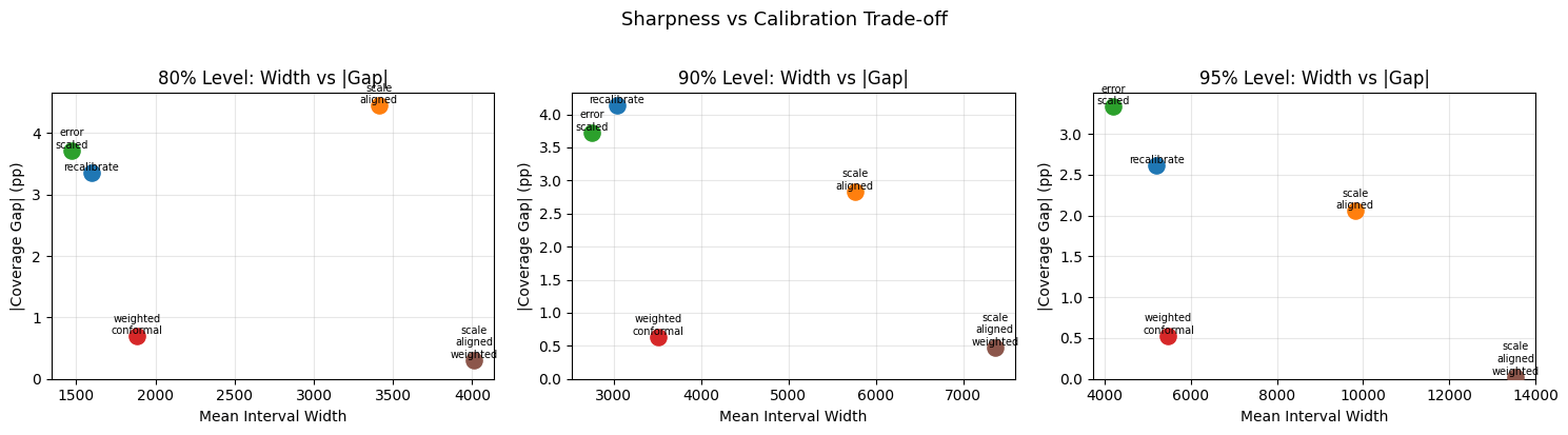
## Interval Width Analysis
Beyond coverage, we also care about interval sharpness. Narrower
intervals (lower width) are better, as long as coverage is maintained.
```python theme={null}
width_results = {}
for method in transfer_methods:
preds = mlf.predict(
h=HORIZON,
level=LEVELS,
new_df=target_train,
transfer_conformal=method,
)
widths = {}
for lv in LEVELS:
lo_col = f'{MODEL}-lo-{lv}'
hi_col = f'{MODEL}-hi-{lv}'
width = (preds[hi_col] - preds[lo_col]).mean()
widths[lv] = float(width)
width_results[method] = widths
width_df = pd.DataFrame(width_results).T
width_df.columns = [f'{lv}%' for lv in LEVELS]
print("Mean interval width by method and level:")
print(width_df.round(2).to_string())
```
```text theme={null}
Mean interval width by method and level:
80% 90% 95%
recalibrate 1596.68 3038.93 5199.22
scale_aligned 3410.02 5759.49 9812.96
error_scaled 1469.70 2755.49 4186.24
weighted_conformal 1883.55 3512.86 5472.55
scale_aligned_weighted 4012.52 7362.65 13545.20
```
```python theme={null}
# Scatter plot: width vs coverage gap (ideal: small gap, narrow width)
fig, axes = plt.subplots(1, 3, figsize=(15, 4))
colors = plt.cm.tab10(np.linspace(0, 0.5, len(transfer_methods)))
for ax, lv in zip(axes, LEVELS):
for i, method in enumerate(transfer_methods):
gap = abs(coverage_results[method][lv] - lv / 100) * 100
width = width_results[method][lv]
ax.scatter(width, gap, color=colors[i], s=120, label=method, zorder=3)
ax.annotate(
method.replace('_', '\n'),
(width, gap), fontsize=7, ha='center', va='bottom'
)
ax.set_xlabel('Mean Interval Width')
ax.set_ylabel('|Coverage Gap| (pp)')
ax.set_title(f'{lv}% Level: Width vs |Gap|')
ax.set_ylim(bottom=0)
ax.grid(True, alpha=0.3)
plt.suptitle('Sharpness vs Calibration Trade-off', fontsize=13, y=1.02)
plt.tight_layout()
plt.show()
```
## Coverage Gap Analysis
```python theme={null}
# Signed gap: positive = over-coverage, negative = under-coverage
gap_pivot = results_df.pivot(index='Method', columns='Nominal Level', values='Gap')[['80%', '90%', '95%']]
gap_display = (gap_pivot * 100).round(2)
print("Coverage gap (Empirical − Nominal) in percentage points:")
print(" Positive = over-coverage (wider intervals than needed)")
print(" Negative = under-coverage (intervals too narrow)")
print()
print(gap_display.to_string())
# Best method: smallest mean absolute gap across all levels
mean_abs_gap = gap_pivot.abs().mean(axis=1).sort_values()
print("\nMethods ranked by mean |gap| across all levels:")
for method, gap in mean_abs_gap.items():
print(f" {method}: {gap*100:.2f} pp")
```
```text theme={null}
Coverage gap (Empirical − Nominal) in percentage points:
Positive = over-coverage (wider intervals than needed)
Negative = under-coverage (intervals too narrow)
Nominal Level 80% 90% 95%
Method
error_scaled -3.72 -3.72 -3.33
recalibrate -3.36 -4.14 -2.61
scale_aligned -4.44 -2.83 -2.06
scale_aligned_weighted -0.31 0.47 0.03
weighted_conformal 0.69 -0.64 -0.53
Methods ranked by mean |gap| across all levels:
scale_aligned_weighted: 0.27 pp
weighted_conformal: 0.62 pp
scale_aligned: 3.11 pp
recalibrate: 3.37 pp
error_scaled: 3.59 pp
```
## Interval Width Analysis
Beyond coverage, we also care about interval sharpness. Narrower
intervals (lower width) are better, as long as coverage is maintained.
```python theme={null}
width_results = {}
for method in transfer_methods:
preds = mlf.predict(
h=HORIZON,
level=LEVELS,
new_df=target_train,
transfer_conformal=method,
)
widths = {}
for lv in LEVELS:
lo_col = f'{MODEL}-lo-{lv}'
hi_col = f'{MODEL}-hi-{lv}'
width = (preds[hi_col] - preds[lo_col]).mean()
widths[lv] = float(width)
width_results[method] = widths
width_df = pd.DataFrame(width_results).T
width_df.columns = [f'{lv}%' for lv in LEVELS]
print("Mean interval width by method and level:")
print(width_df.round(2).to_string())
```
```text theme={null}
Mean interval width by method and level:
80% 90% 95%
recalibrate 1596.68 3038.93 5199.22
scale_aligned 3410.02 5759.49 9812.96
error_scaled 1469.70 2755.49 4186.24
weighted_conformal 1883.55 3512.86 5472.55
scale_aligned_weighted 4012.52 7362.65 13545.20
```
```python theme={null}
# Scatter plot: width vs coverage gap (ideal: small gap, narrow width)
fig, axes = plt.subplots(1, 3, figsize=(15, 4))
colors = plt.cm.tab10(np.linspace(0, 0.5, len(transfer_methods)))
for ax, lv in zip(axes, LEVELS):
for i, method in enumerate(transfer_methods):
gap = abs(coverage_results[method][lv] - lv / 100) * 100
width = width_results[method][lv]
ax.scatter(width, gap, color=colors[i], s=120, label=method, zorder=3)
ax.annotate(
method.replace('_', '\n'),
(width, gap), fontsize=7, ha='center', va='bottom'
)
ax.set_xlabel('Mean Interval Width')
ax.set_ylabel('|Coverage Gap| (pp)')
ax.set_title(f'{lv}% Level: Width vs |Gap|')
ax.set_ylim(bottom=0)
ax.grid(True, alpha=0.3)
plt.suptitle('Sharpness vs Calibration Trade-off', fontsize=13, y=1.02)
plt.tight_layout()
plt.show()
```
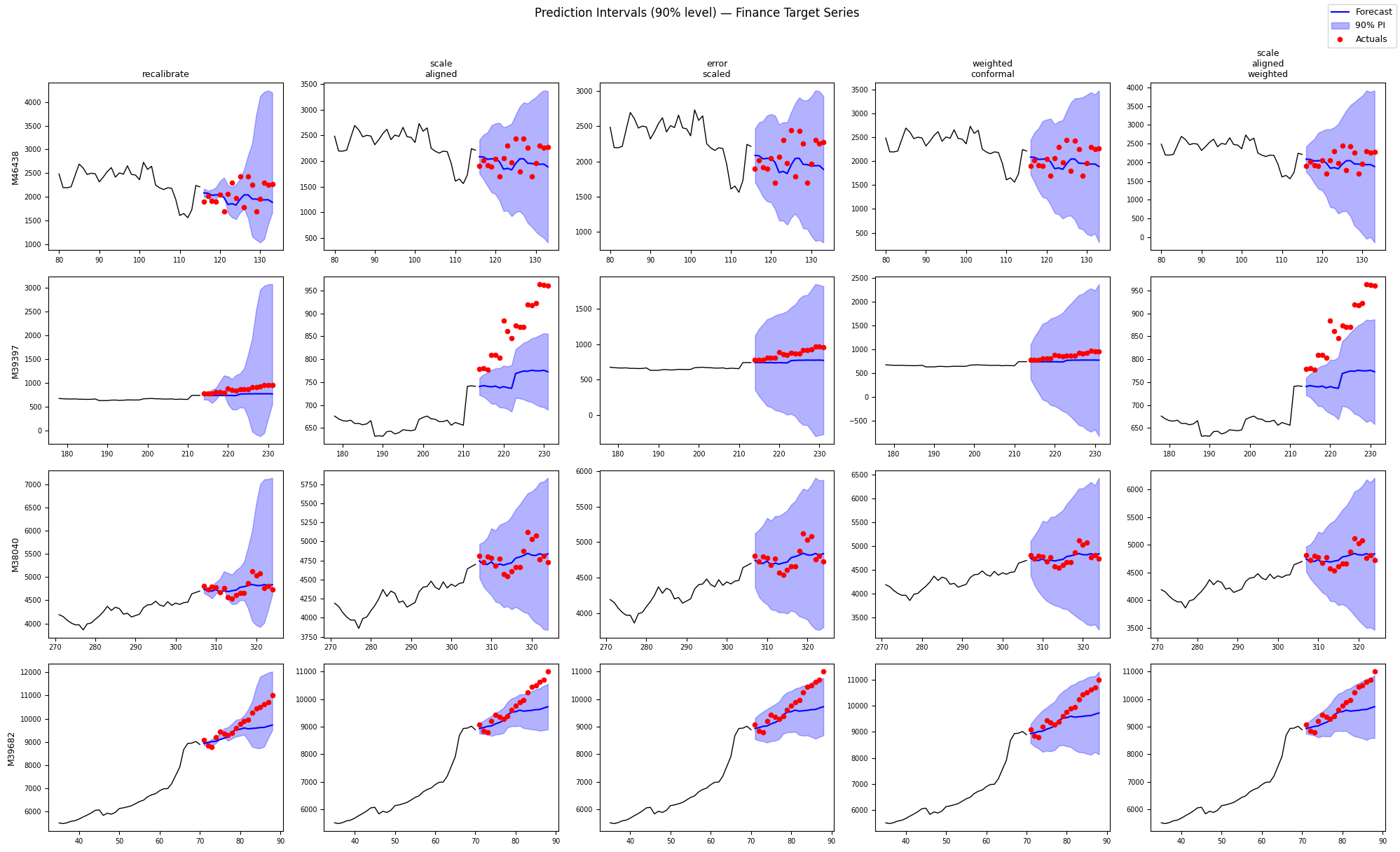
 ## Visual Inspection: Interval Examples
Let’s visually inspect the intervals produced by each method for a few
target-domain series.
```python theme={null}
PLOT_LEVEL = 90
EXAMPLE_IDS = target_ids[:4].tolist()
# Collect predictions for all methods
all_preds = {}
for method in transfer_methods:
preds = mlf.predict(
h=HORIZON,
level=[PLOT_LEVEL],
new_df=target_train[target_train['unique_id'].isin(EXAMPLE_IDS)],
transfer_conformal=method,
)
all_preds[method] = preds
```
```python theme={null}
fig, axes = plt.subplots(
len(EXAMPLE_IDS), len(transfer_methods),
figsize=(4 * len(transfer_methods), 3 * len(EXAMPLE_IDS)),
sharex='row'
)
lo_col = f'{MODEL}-lo-{PLOT_LEVEL}'
hi_col = f'{MODEL}-hi-{PLOT_LEVEL}'
for row, uid in enumerate(EXAMPLE_IDS):
hist = target_train[target_train['unique_id'] == uid].tail(36)
test = target_test[target_test['unique_id'] == uid]
for col, method in enumerate(transfer_methods):
ax = axes[row][col]
pred = all_preds[method][all_preds[method]['unique_id'] == uid]
ax.plot(hist['ds'], hist['y'], color='black', linewidth=1)
ax.plot(pred['ds'], pred[MODEL], color='blue', linewidth=1.5, label='Forecast')
ax.fill_between(
pred['ds'], pred[lo_col], pred[hi_col],
alpha=0.3, color='blue', label=f'{PLOT_LEVEL}% PI'
)
ax.scatter(test['ds'], test['y'], color='red', s=20, zorder=5, label='Actuals')
if row == 0:
ax.set_title(method.replace('_', '\n'), fontsize=9)
if col == 0:
ax.set_ylabel(f'{uid}', fontsize=9)
ax.tick_params(labelsize=7)
# Single legend at top
handles, labels = axes[0][0].get_legend_handles_labels()
fig.legend(handles, labels, loc='upper right', fontsize=9)
plt.suptitle(
f'Prediction Intervals ({PLOT_LEVEL}% level) — Finance Target Series',
fontsize=12, y=1.01
)
plt.tight_layout()
plt.show()
```
## Visual Inspection: Interval Examples
Let’s visually inspect the intervals produced by each method for a few
target-domain series.
```python theme={null}
PLOT_LEVEL = 90
EXAMPLE_IDS = target_ids[:4].tolist()
# Collect predictions for all methods
all_preds = {}
for method in transfer_methods:
preds = mlf.predict(
h=HORIZON,
level=[PLOT_LEVEL],
new_df=target_train[target_train['unique_id'].isin(EXAMPLE_IDS)],
transfer_conformal=method,
)
all_preds[method] = preds
```
```python theme={null}
fig, axes = plt.subplots(
len(EXAMPLE_IDS), len(transfer_methods),
figsize=(4 * len(transfer_methods), 3 * len(EXAMPLE_IDS)),
sharex='row'
)
lo_col = f'{MODEL}-lo-{PLOT_LEVEL}'
hi_col = f'{MODEL}-hi-{PLOT_LEVEL}'
for row, uid in enumerate(EXAMPLE_IDS):
hist = target_train[target_train['unique_id'] == uid].tail(36)
test = target_test[target_test['unique_id'] == uid]
for col, method in enumerate(transfer_methods):
ax = axes[row][col]
pred = all_preds[method][all_preds[method]['unique_id'] == uid]
ax.plot(hist['ds'], hist['y'], color='black', linewidth=1)
ax.plot(pred['ds'], pred[MODEL], color='blue', linewidth=1.5, label='Forecast')
ax.fill_between(
pred['ds'], pred[lo_col], pred[hi_col],
alpha=0.3, color='blue', label=f'{PLOT_LEVEL}% PI'
)
ax.scatter(test['ds'], test['y'], color='red', s=20, zorder=5, label='Actuals')
if row == 0:
ax.set_title(method.replace('_', '\n'), fontsize=9)
if col == 0:
ax.set_ylabel(f'{uid}', fontsize=9)
ax.tick_params(labelsize=7)
# Single legend at top
handles, labels = axes[0][0].get_legend_handles_labels()
fig.legend(handles, labels, loc='upper right', fontsize=9)
plt.suptitle(
f'Prediction Intervals ({PLOT_LEVEL}% level) — Finance Target Series',
fontsize=12, y=1.01
)
plt.tight_layout()
plt.show()
```
 ## Summary
The table and charts above show how each transfer method calibrates
prediction intervals when moving from a Macro source domain to a Finance
target domain in M4 Monthly data.
**Key takeaways:**
* **Feature engineering matters as much as the transfer method.**
Modeling log-returns (`log1p` + `Differences([1])`) instead of raw
differences makes the features scale-invariant across domains,
removes the systematic point-forecast bias, and is what allows the
weighted methods to reach near-nominal coverage. With raw
differences, every method under-covers by several percentage points.
* `recalibrate` runs cross-validation on the target data — it tends to
be the most directly calibrated but requires running CV
(computationally equivalent to retraining).
* `scale_aligned` uses the scale of the *y* signal (MAD of
differences) to align source residuals — zero-shot, no CV needed.
* `error_scaled` runs CV on the target data to estimate prediction
error magnitude — a middle ground between full recalibration and
scale alignment.
* `weighted_conformal` uses density-ratio estimation to reweight
source conformity scores — handles covariate shift without needing
target labels during calibration.
* `scale_aligned_weighted` combines scale alignment with DRE weighting
— the most sophisticated zero-shot method.
* The residual under-coverage of the non-weighted methods comes from
pooling conformity scores across heterogeneous series: pooled
intervals are too wide for calm series and too narrow for volatile
ones. This is precisely the failure mode the weighted/scale-aligned
variants are designed to mitigate.
The right method to use depends on your constraints: - If you can run CV
on the target: `recalibrate` or `error_scaled` - If you need zero-shot
transfer: `scale_aligned` or `scale_aligned_weighted` - If covariate
shift is the main concern: `weighted_conformal` or
`scale_aligned_weighted`
## Summary
The table and charts above show how each transfer method calibrates
prediction intervals when moving from a Macro source domain to a Finance
target domain in M4 Monthly data.
**Key takeaways:**
* **Feature engineering matters as much as the transfer method.**
Modeling log-returns (`log1p` + `Differences([1])`) instead of raw
differences makes the features scale-invariant across domains,
removes the systematic point-forecast bias, and is what allows the
weighted methods to reach near-nominal coverage. With raw
differences, every method under-covers by several percentage points.
* `recalibrate` runs cross-validation on the target data — it tends to
be the most directly calibrated but requires running CV
(computationally equivalent to retraining).
* `scale_aligned` uses the scale of the *y* signal (MAD of
differences) to align source residuals — zero-shot, no CV needed.
* `error_scaled` runs CV on the target data to estimate prediction
error magnitude — a middle ground between full recalibration and
scale alignment.
* `weighted_conformal` uses density-ratio estimation to reweight
source conformity scores — handles covariate shift without needing
target labels during calibration.
* `scale_aligned_weighted` combines scale alignment with DRE weighting
— the most sophisticated zero-shot method.
* The residual under-coverage of the non-weighted methods comes from
pooling conformity scores across heterogeneous series: pooled
intervals are too wide for calm series and too narrow for volatile
ones. This is precisely the failure mode the weighted/scale-aligned
variants are designed to mitigate.
The right method to use depends on your constraints: - If you can run CV
on the target: `recalibrate` or `error_scaled` - If you need zero-shot
transfer: `scale_aligned` or `scale_aligned_weighted` - If covariate
shift is the main concern: `weighted_conformal` or
`scale_aligned_weighted`