> ## Documentation Index
> Fetch the complete documentation index at: https://nixtlaverse.nixtla.io/llms.txt
> Use this file to discover all available pages before exploring further.
# M4 Competition
This shows an example with just 4 series of the M4 dataset. If you want
to run it yourself on all of them, you can refer to [this
notebook](https://www.kaggle.com/code/lemuz90/m4-competition).
```python theme={null}
import random
import lightgbm as lgb
import numpy as np
import pandas as pd
from sklearn.linear_model import LinearRegression
from utilsforecast.plotting import plot_series
from mlforecast import MLForecast
from mlforecast.lag_transforms import (
ExponentiallyWeightedMean,
RollingMean,
)
from mlforecast.lgb_cv import LightGBMCV
from mlforecast.target_transforms import Differences
from mlforecast.utils import PredictionIntervals
```
```python theme={null}
df = pd.read_parquet('https://datasets-nixtla.s3.amazonaws.com/m4-hourly.parquet')
ids = df['unique_id'].unique()
random.seed(0)
sample_ids = random.choices(ids, k=4)
sample_df = df[df['unique_id'].isin(sample_ids)]
sample_df
```
| | unique\_id | ds | y |
| ------ | ---------- | ---- | ---- |
| 86796 | H196 | 1 | 11.8 |
| 86797 | H196 | 2 | 11.4 |
| 86798 | H196 | 3 | 11.1 |
| 86799 | H196 | 4 | 10.8 |
| 86800 | H196 | 5 | 10.6 |
| ... | ... | ... | ... |
| 325235 | H413 | 1004 | 99.0 |
| 325236 | H413 | 1005 | 88.0 |
| 325237 | H413 | 1006 | 47.0 |
| 325238 | H413 | 1007 | 41.0 |
| 325239 | H413 | 1008 | 34.0 |
We now split this data into train and validation.
```python theme={null}
horizon = 48
valid = sample_df.groupby('unique_id').tail(horizon)
train = sample_df.drop(valid.index)
train.shape, valid.shape
```
```text theme={null}
((3840, 3), (192, 3))
```
## Creating the forecaster
```python theme={null}
fcst = MLForecast(
models=lgb.LGBMRegressor(random_state=0, verbosity=-1),
freq=1,
lags=[24 * (i+1) for i in range(7)],
lag_transforms={
48: [ExponentiallyWeightedMean(alpha=0.3)],
},
num_threads=1,
target_transforms=[Differences([24])],
)
```
```python theme={null}
fcst
```
```text theme={null}
MLForecast(models=[LGBMRegressor], freq=1, lag_features=['lag24', 'lag48', 'lag72', 'lag96', 'lag120', 'lag144', 'lag168', 'exponentially_weighted_mean_lag48_alpha0.3'], date_features=[], num_threads=1)
```
Once we have this setup we can compute the features and fit the model.
## Fitting and predicting
```python theme={null}
fcst = MLForecast(
models=lgb.LGBMRegressor(random_state=0, verbosity=-1),
freq=1,
lags=[24 * (i+1) for i in range(7)],
lag_transforms={
48: [ExponentiallyWeightedMean(alpha=0.3)],
},
num_threads=1,
target_transforms=[Differences([24])],
)
```
```python theme={null}
train2 = train.copy()
train2['weight'] = np.random.default_rng(seed=0).random(train2.shape[0])
fcst.fit(train2, weight_col='weight', as_numpy=True).predict(5)
```
| | unique\_id | ds | LGBMRegressor |
| -- | ---------- | --- | ------------- |
| 0 | H196 | 961 | 16.079737 |
| 1 | H196 | 962 | 15.679737 |
| 2 | H196 | 963 | 15.279737 |
| 3 | H196 | 964 | 14.979737 |
| 4 | H196 | 965 | 14.679737 |
| 5 | H256 | 961 | 13.279737 |
| 6 | H256 | 962 | 12.679737 |
| 7 | H256 | 963 | 12.379737 |
| 8 | H256 | 964 | 12.079737 |
| 9 | H256 | 965 | 11.879737 |
| 10 | H381 | 961 | 56.939977 |
| 11 | H381 | 962 | 40.314608 |
| 12 | H381 | 963 | 33.859013 |
| 13 | H381 | 964 | 15.498139 |
| 14 | H381 | 965 | 25.722674 |
| 15 | H413 | 961 | 25.131194 |
| 16 | H413 | 962 | 19.177421 |
| 17 | H413 | 963 | 21.250829 |
| 18 | H413 | 964 | 18.743132 |
| 19 | H413 | 965 | 16.027263 |
```python theme={null}
fcst.cross_validation(train2, n_windows=2, h=5, weight_col='weight', as_numpy=True)
```
| | unique\_id | ds | cutoff | y | LGBMRegressor |
| -- | ---------- | --- | ------ | ----- | ------------- |
| 0 | H196 | 951 | 950 | 24.4 | 24.288850 |
| 1 | H196 | 952 | 950 | 24.3 | 24.188850 |
| 2 | H196 | 953 | 950 | 23.8 | 23.688850 |
| 3 | H196 | 954 | 950 | 22.8 | 22.688850 |
| 4 | H196 | 955 | 950 | 21.2 | 21.088850 |
| 5 | H256 | 951 | 950 | 19.5 | 19.688850 |
| 6 | H256 | 952 | 950 | 19.4 | 19.488850 |
| 7 | H256 | 953 | 950 | 18.9 | 19.088850 |
| 8 | H256 | 954 | 950 | 18.3 | 18.388850 |
| 9 | H256 | 955 | 950 | 17.0 | 17.088850 |
| 10 | H381 | 951 | 950 | 182.0 | 208.327270 |
| 11 | H381 | 952 | 950 | 222.0 | 247.768326 |
| 12 | H381 | 953 | 950 | 288.0 | 277.965997 |
| 13 | H381 | 954 | 950 | 264.0 | 321.532857 |
| 14 | H381 | 955 | 950 | 191.0 | 206.316903 |
| 15 | H413 | 951 | 950 | 77.0 | 60.972692 |
| 16 | H413 | 952 | 950 | 91.0 | 54.936494 |
| 17 | H413 | 953 | 950 | 76.0 | 73.949203 |
| 18 | H413 | 954 | 950 | 68.0 | 67.087417 |
| 19 | H413 | 955 | 950 | 68.0 | 75.896022 |
| 20 | H196 | 956 | 955 | 19.3 | 19.287891 |
| 21 | H196 | 957 | 955 | 18.2 | 18.187891 |
| 22 | H196 | 958 | 955 | 17.5 | 17.487891 |
| 23 | H196 | 959 | 955 | 16.9 | 16.887891 |
| 24 | H196 | 960 | 955 | 16.5 | 16.487891 |
| 25 | H256 | 956 | 955 | 15.5 | 15.687891 |
| 26 | H256 | 957 | 955 | 14.7 | 14.787891 |
| 27 | H256 | 958 | 955 | 14.1 | 14.287891 |
| 28 | H256 | 959 | 955 | 13.6 | 13.787891 |
| 29 | H256 | 960 | 955 | 13.2 | 13.387891 |
| 30 | H381 | 956 | 955 | 130.0 | 124.117828 |
| 31 | H381 | 957 | 955 | 113.0 | 119.180350 |
| 32 | H381 | 958 | 955 | 94.0 | 105.356552 |
| 33 | H381 | 959 | 955 | 192.0 | 127.095338 |
| 34 | H381 | 960 | 955 | 87.0 | 119.875754 |
| 35 | H413 | 956 | 955 | 59.0 | 67.993133 |
| 36 | H413 | 957 | 955 | 58.0 | 69.869815 |
| 37 | H413 | 958 | 955 | 53.0 | 34.717960 |
| 38 | H413 | 959 | 955 | 38.0 | 47.665581 |
| 39 | H413 | 960 | 955 | 46.0 | 45.940137 |
```python theme={null}
fcst.fit(train, fitted=True);
```
```python theme={null}
expected_future = fcst.make_future_dataframe(h=1)
expected_future
```
| | unique\_id | ds |
| - | ---------- | --- |
| 0 | H196 | 961 |
| 1 | H256 | 961 |
| 2 | H381 | 961 |
| 3 | H413 | 961 |
```python theme={null}
missing_future = fcst.get_missing_future(h=1, X_df=expected_future.head(2))
pd.testing.assert_frame_equal(
missing_future,
expected_future.tail(2).reset_index(drop=True)
)
```
```python theme={null}
fcst.forecast_fitted_values()
```
| | unique\_id | ds | y | LGBMRegressor |
| ---- | ---------- | --- | ---- | ------------- |
| 0 | H196 | 193 | 12.7 | 12.671271 |
| 1 | H196 | 194 | 12.3 | 12.271271 |
| 2 | H196 | 195 | 11.9 | 11.871271 |
| 3 | H196 | 196 | 11.7 | 11.671271 |
| 4 | H196 | 197 | 11.4 | 11.471271 |
| ... | ... | ... | ... | ... |
| 3067 | H413 | 956 | 59.0 | 68.280574 |
| 3068 | H413 | 957 | 58.0 | 70.427570 |
| 3069 | H413 | 958 | 53.0 | 44.767965 |
| 3070 | H413 | 959 | 38.0 | 48.691257 |
| 3071 | H413 | 960 | 46.0 | 46.652238 |
```python theme={null}
fcst.forecast_fitted_values(level=[90])
```
| | unique\_id | ds | y | LGBMRegressor | LGBMRegressor-lo-90 | LGBMRegressor-hi-90 |
| ---- | ---------- | --- | ---- | ------------- | ------------------- | ------------------- |
| 0 | H196 | 193 | 12.7 | 12.671271 | 12.540634 | 12.801909 |
| 1 | H196 | 194 | 12.3 | 12.271271 | 12.140634 | 12.401909 |
| 2 | H196 | 195 | 11.9 | 11.871271 | 11.740634 | 12.001909 |
| 3 | H196 | 196 | 11.7 | 11.671271 | 11.540634 | 11.801909 |
| 4 | H196 | 197 | 11.4 | 11.471271 | 11.340634 | 11.601909 |
| ... | ... | ... | ... | ... | ... | ... |
| 3067 | H413 | 956 | 59.0 | 68.280574 | 58.846640 | 77.714509 |
| 3068 | H413 | 957 | 58.0 | 70.427570 | 60.993636 | 79.861504 |
| 3069 | H413 | 958 | 53.0 | 44.767965 | 35.334031 | 54.201899 |
| 3070 | H413 | 959 | 38.0 | 48.691257 | 39.257323 | 58.125191 |
| 3071 | H413 | 960 | 46.0 | 46.652238 | 37.218304 | 56.086172 |
Once we’ve run this we’re ready to compute our predictions.
```python theme={null}
predictions = fcst.predict(horizon)
```
We can see at a couple of results.
```python theme={null}
results = valid.merge(predictions, on=['unique_id', 'ds'])
fig = plot_series(forecasts_df=results)
```
```python theme={null}
fig
```
 ### Prediction intervals
With
[`MLForecast`](https://Nixtla.github.io/mlforecast/forecast.html#mlforecast),
you can generate prediction intervals using Conformal Prediction. To
configure Conformal Prediction, you need to pass an instance of the
[`PredictionIntervals`](https://Nixtla.github.io/mlforecast/utils.html#predictionintervals)
class to the `prediction_intervals` argument of the `fit` method. The
class takes three parameters: `n_windows`, `h` and `method`.
* `n_windows` represents the number of cross-validation windows used
to calibrate the intervals
* `h` is the forecast horizon
* `method` can be `conformal_distribution` or `conformal_error`;
`conformal_distribution` (default) creates forecasts paths based on
the cross-validation errors and calculate quantiles using those
paths, on the other hand `conformal_error` calculates the error
quantiles to produce prediction intervals. The strategy will adjust
the intervals for each horizon step, resulting in different widths
for each step. Please note that a minimum of 2 cross-validation
windows must be used.
```python theme={null}
fcst.fit(
train,
prediction_intervals=PredictionIntervals(n_windows=3, h=48)
)
```
```text theme={null}
MLForecast(models=[LGBMRegressor], freq=1, lag_features=['lag24', 'lag48', 'lag72', 'lag96', 'lag120', 'lag144', 'lag168', 'exponentially_weighted_mean_lag48_alpha0.3'], date_features=[], num_threads=1)
```
After that, you just have to include your desired confidence levels to
the `predict` method using the `level` argument. Levels must lie between
0 and 100.
```python theme={null}
predictions_w_intervals = fcst.predict(48, level=[50, 80, 95])
predictions_w_intervals.head()
```
| | unique\_id | ds | LGBMRegressor | LGBMRegressor-lo-95 | LGBMRegressor-lo-80 | LGBMRegressor-lo-50 | LGBMRegressor-hi-50 | LGBMRegressor-hi-80 | LGBMRegressor-hi-95 |
| - | ---------- | --- | ------------- | ------------------- | ------------------- | ------------------- | ------------------- | ------------------- | ------------------- |
| 0 | H196 | 961 | 16.071271 | 15.958042 | 15.971271 | 16.005091 | 16.137452 | 16.171271 | 16.184501 |
| 1 | H196 | 962 | 15.671271 | 15.553632 | 15.553632 | 15.578632 | 15.763911 | 15.788911 | 15.788911 |
| 2 | H196 | 963 | 15.271271 | 15.153632 | 15.153632 | 15.162452 | 15.380091 | 15.388911 | 15.388911 |
| 3 | H196 | 964 | 14.971271 | 14.858042 | 14.871271 | 14.905091 | 15.037452 | 15.071271 | 15.084501 |
| 4 | H196 | 965 | 14.671271 | 14.553632 | 14.553632 | 14.562452 | 14.780091 | 14.788911 | 14.788911 |
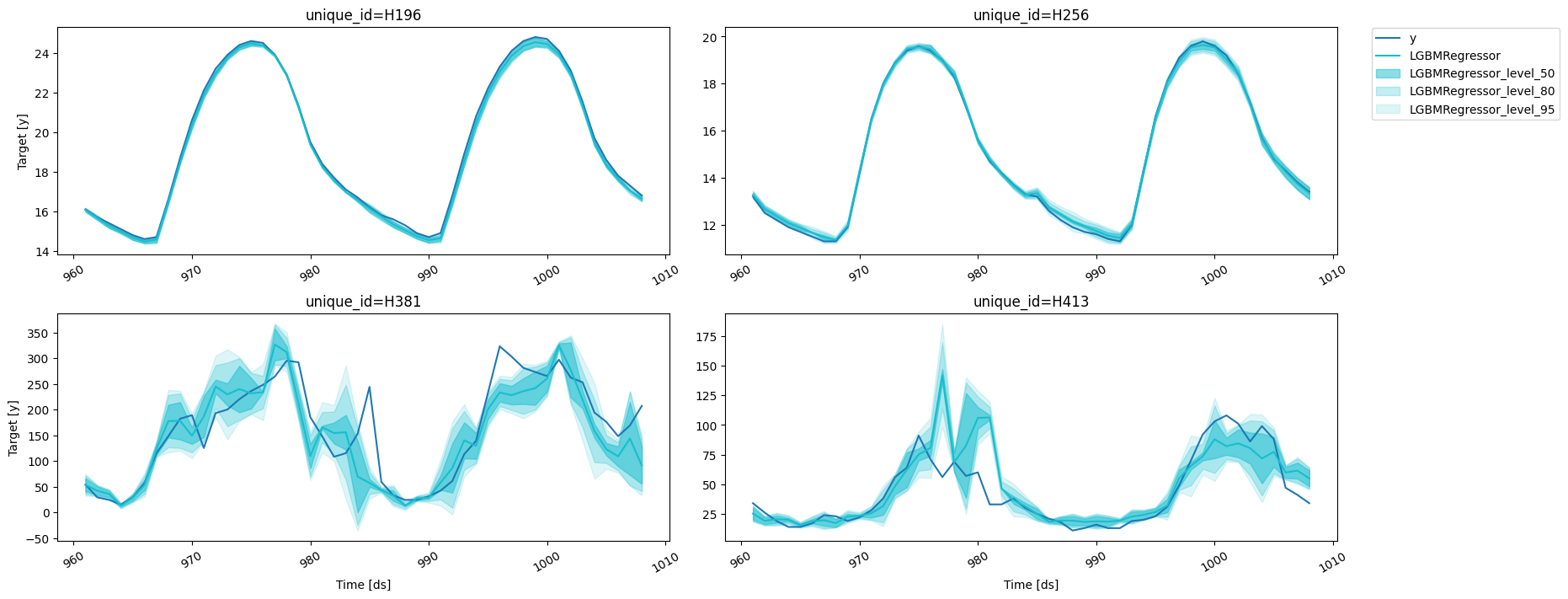
Let’s explore the generated intervals.
```python theme={null}
results = valid.merge(predictions_w_intervals, on=['unique_id', 'ds'])
fig = plot_series(forecasts_df=results, level=[50, 80, 95])
fig
```
### Prediction intervals
With
[`MLForecast`](https://Nixtla.github.io/mlforecast/forecast.html#mlforecast),
you can generate prediction intervals using Conformal Prediction. To
configure Conformal Prediction, you need to pass an instance of the
[`PredictionIntervals`](https://Nixtla.github.io/mlforecast/utils.html#predictionintervals)
class to the `prediction_intervals` argument of the `fit` method. The
class takes three parameters: `n_windows`, `h` and `method`.
* `n_windows` represents the number of cross-validation windows used
to calibrate the intervals
* `h` is the forecast horizon
* `method` can be `conformal_distribution` or `conformal_error`;
`conformal_distribution` (default) creates forecasts paths based on
the cross-validation errors and calculate quantiles using those
paths, on the other hand `conformal_error` calculates the error
quantiles to produce prediction intervals. The strategy will adjust
the intervals for each horizon step, resulting in different widths
for each step. Please note that a minimum of 2 cross-validation
windows must be used.
```python theme={null}
fcst.fit(
train,
prediction_intervals=PredictionIntervals(n_windows=3, h=48)
)
```
```text theme={null}
MLForecast(models=[LGBMRegressor], freq=1, lag_features=['lag24', 'lag48', 'lag72', 'lag96', 'lag120', 'lag144', 'lag168', 'exponentially_weighted_mean_lag48_alpha0.3'], date_features=[], num_threads=1)
```
After that, you just have to include your desired confidence levels to
the `predict` method using the `level` argument. Levels must lie between
0 and 100.
```python theme={null}
predictions_w_intervals = fcst.predict(48, level=[50, 80, 95])
predictions_w_intervals.head()
```
| | unique\_id | ds | LGBMRegressor | LGBMRegressor-lo-95 | LGBMRegressor-lo-80 | LGBMRegressor-lo-50 | LGBMRegressor-hi-50 | LGBMRegressor-hi-80 | LGBMRegressor-hi-95 |
| - | ---------- | --- | ------------- | ------------------- | ------------------- | ------------------- | ------------------- | ------------------- | ------------------- |
| 0 | H196 | 961 | 16.071271 | 15.958042 | 15.971271 | 16.005091 | 16.137452 | 16.171271 | 16.184501 |
| 1 | H196 | 962 | 15.671271 | 15.553632 | 15.553632 | 15.578632 | 15.763911 | 15.788911 | 15.788911 |
| 2 | H196 | 963 | 15.271271 | 15.153632 | 15.153632 | 15.162452 | 15.380091 | 15.388911 | 15.388911 |
| 3 | H196 | 964 | 14.971271 | 14.858042 | 14.871271 | 14.905091 | 15.037452 | 15.071271 | 15.084501 |
| 4 | H196 | 965 | 14.671271 | 14.553632 | 14.553632 | 14.562452 | 14.780091 | 14.788911 | 14.788911 |
Let’s explore the generated intervals.
```python theme={null}
results = valid.merge(predictions_w_intervals, on=['unique_id', 'ds'])
fig = plot_series(forecasts_df=results, level=[50, 80, 95])
fig
```
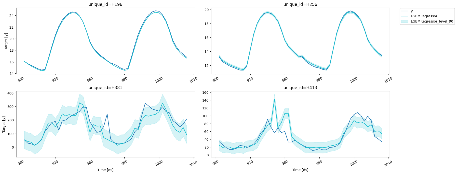
 If you want to reduce the computational time and produce intervals with
the same width for the whole forecast horizon, simple pass `h=1` to the
[`PredictionIntervals`](https://Nixtla.github.io/mlforecast/utils.html#predictionintervals)
class. The caveat of this strategy is that in some cases, variance of
the absolute residuals maybe be small (even zero), so the intervals may
be too narrow.
```python theme={null}
fcst.fit(
train,
prediction_intervals=PredictionIntervals(n_windows=3, h=1)
);
```
```python theme={null}
predictions_w_intervals_ws_1 = fcst.predict(48, level=[80, 90, 95])
```
Let’s explore the generated intervals.
```python theme={null}
results = valid.merge(predictions_w_intervals_ws_1, on=['unique_id', 'ds'])
fig = plot_series(forecasts_df=results, level=[90])
fig
```
If you want to reduce the computational time and produce intervals with
the same width for the whole forecast horizon, simple pass `h=1` to the
[`PredictionIntervals`](https://Nixtla.github.io/mlforecast/utils.html#predictionintervals)
class. The caveat of this strategy is that in some cases, variance of
the absolute residuals maybe be small (even zero), so the intervals may
be too narrow.
```python theme={null}
fcst.fit(
train,
prediction_intervals=PredictionIntervals(n_windows=3, h=1)
);
```
```python theme={null}
predictions_w_intervals_ws_1 = fcst.predict(48, level=[80, 90, 95])
```
Let’s explore the generated intervals.
```python theme={null}
results = valid.merge(predictions_w_intervals_ws_1, on=['unique_id', 'ds'])
fig = plot_series(forecasts_df=results, level=[90])
fig
```
 ### Forecast using a pretrained model
MLForecast allows you to use a pretrained model to generate forecasts
for a new dataset. Simply provide a pandas dataframe containing the new
observations as the value for the `new_df` argument when calling the
`predict` method. The dataframe should have the same structure as the
one used to fit the model, including any features and time series data.
The function will then use the pretrained model to generate forecasts
for the new observations. This allows you to easily apply a pretrained
model to a new dataset and generate forecasts without the need to
retrain the model.
```python theme={null}
ercot_df = pd.read_csv('https://datasets-nixtla.s3.amazonaws.com/ERCOT-clean.csv')
# we have to convert the ds column to integers
# since MLForecast was trained with that structure
ercot_df['ds'] = np.arange(1, len(ercot_df) + 1)
# use the `new_df` argument to pass the ercot dataset
ercot_fcsts = fcst.predict(horizon, new_df=ercot_df)
fig = plot_series(ercot_df, ercot_fcsts, max_insample_length=48 * 2)
fig
```
### Forecast using a pretrained model
MLForecast allows you to use a pretrained model to generate forecasts
for a new dataset. Simply provide a pandas dataframe containing the new
observations as the value for the `new_df` argument when calling the
`predict` method. The dataframe should have the same structure as the
one used to fit the model, including any features and time series data.
The function will then use the pretrained model to generate forecasts
for the new observations. This allows you to easily apply a pretrained
model to a new dataset and generate forecasts without the need to
retrain the model.
```python theme={null}
ercot_df = pd.read_csv('https://datasets-nixtla.s3.amazonaws.com/ERCOT-clean.csv')
# we have to convert the ds column to integers
# since MLForecast was trained with that structure
ercot_df['ds'] = np.arange(1, len(ercot_df) + 1)
# use the `new_df` argument to pass the ercot dataset
ercot_fcsts = fcst.predict(horizon, new_df=ercot_df)
fig = plot_series(ercot_df, ercot_fcsts, max_insample_length=48 * 2)
fig
```
 ### Preprocess
If you want to take a look at the data that will be used to train the
models you can call `Forecast.preprocess`.
```python theme={null}
prep_df = fcst.preprocess(train)
prep_df
```
| | unique\_id | ds | y | lag24 | lag48 | lag72 | lag96 | lag120 | lag144 | lag168 | exponentially\_weighted\_mean\_lag48\_alpha0.3 |
| ------ | ---------- | --- | ---- | ----- | ----- | ----- | ----- | ------ | ------ | ------ | ---------------------------------------------- |
| 86988 | H196 | 193 | 0.1 | 0.0 | 0.0 | 0.0 | 0.3 | 0.1 | 0.1 | 0.3 | 0.002810 |
| 86989 | H196 | 194 | 0.1 | -0.1 | 0.1 | 0.0 | 0.3 | 0.1 | 0.1 | 0.3 | 0.031967 |
| 86990 | H196 | 195 | 0.1 | -0.1 | 0.1 | 0.0 | 0.3 | 0.1 | 0.2 | 0.1 | 0.052377 |
| 86991 | H196 | 196 | 0.1 | 0.0 | 0.0 | 0.0 | 0.3 | 0.2 | 0.1 | 0.2 | 0.036664 |
| 86992 | H196 | 197 | 0.0 | 0.0 | 0.0 | 0.1 | 0.2 | 0.2 | 0.1 | 0.2 | 0.025665 |
| ... | ... | ... | ... | ... | ... | ... | ... | ... | ... | ... | ... |
| 325187 | H413 | 956 | 0.0 | 10.0 | 1.0 | 6.0 | -53.0 | 44.0 | -21.0 | 21.0 | 7.963225 |
| 325188 | H413 | 957 | 9.0 | 10.0 | 10.0 | -7.0 | -46.0 | 27.0 | -19.0 | 24.0 | 8.574257 |
| 325189 | H413 | 958 | 16.0 | 8.0 | 5.0 | -9.0 | -36.0 | 32.0 | -13.0 | 8.0 | 7.501980 |
| 325190 | H413 | 959 | -3.0 | 17.0 | -7.0 | 2.0 | -31.0 | 22.0 | 5.0 | -2.0 | 3.151386 |
| 325191 | H413 | 960 | 15.0 | 11.0 | -6.0 | -5.0 | -17.0 | 22.0 | -18.0 | 10.0 | 0.405970 |
If we do this we then have to call `Forecast.fit_models`, since this
only stores the series information.
```python theme={null}
X, y = prep_df.drop(columns=['unique_id', 'ds', 'y']), prep_df['y']
fcst.fit_models(X, y)
```
```text theme={null}
MLForecast(models=[LGBMRegressor], freq=1, lag_features=['lag24', 'lag48', 'lag72', 'lag96', 'lag120', 'lag144', 'lag168', 'exponentially_weighted_mean_lag48_alpha0.3'], date_features=[], num_threads=1)
```
```python theme={null}
fcst
```
```text theme={null}
MLForecast(models=[LGBMRegressor], freq=1, lag_features=['lag24', 'lag48', 'lag72', 'lag96', 'lag120', 'lag144', 'lag168', 'exponentially_weighted_mean_lag48_alpha0.3'], date_features=[], num_threads=1)
```
```python theme={null}
predictions2 = fcst.predict(horizon)
pd.testing.assert_frame_equal(predictions, predictions2)
```
If we would like to know how good our forecast will be for a specific
model and set of features then we can perform cross validation. What
cross validation does is take our data and split it in two parts, where
the first part is used for training and the second one for validation.
Since the data is time dependant we usually take the last *x*
observations from our data as the validation set.
This process is implemented in
[`MLForecast.cross_validation`](https://Nixtla.github.io/mlforecast/forecast.html#mlforecast.cross_validation),
which takes our data and performs the process described above for
`n_windows` times where each window has `h` validation samples in it.
For example, if we have 100 samples and we want to perform 2 backtests
each of size 14, the splits will be as follows:
1. Train: 1 to 72. Validation: 73 to 86.
2. Train: 1 to 86. Validation: 87 to 100.
You can control the size between each cross validation window using the
`step_size` argument. For example, if we have 100 samples and we want to
perform 2 backtests each of size 14 and move one step ahead in each fold
(`step_size=1`), the splits will be as follows:
1. Train: 1 to 85. Validation: 86 to 99.
2. Train: 1 to 86. Validation: 87 to 100.
You can also perform cross validation without refitting your models for
each window by setting `refit=False`. This allows you to evaluate the
performance of your models using multiple window sizes without having to
retrain them each time.
```python theme={null}
fcst = MLForecast(
models=lgb.LGBMRegressor(random_state=0, verbosity=-1),
freq=1,
lags=[24 * (i+1) for i in range(7)],
lag_transforms={
1: [RollingMean(window_size=24)],
24: [RollingMean(window_size=24)],
48: [ExponentiallyWeightedMean(alpha=0.3)],
},
num_threads=1,
target_transforms=[Differences([24])],
)
cv_results = fcst.cross_validation(
train,
n_windows=2,
h=horizon,
step_size=horizon,
fitted=True,
)
cv_results
```
| | unique\_id | ds | cutoff | y | LGBMRegressor |
| --- | ---------- | --- | ------ | ---- | ------------- |
| 0 | H196 | 865 | 864 | 15.5 | 15.373393 |
| 1 | H196 | 866 | 864 | 15.1 | 14.973393 |
| 2 | H196 | 867 | 864 | 14.8 | 14.673393 |
| 3 | H196 | 868 | 864 | 14.4 | 14.373393 |
| 4 | H196 | 869 | 864 | 14.2 | 14.073393 |
| ... | ... | ... | ... | ... | ... |
| 379 | H413 | 956 | 912 | 59.0 | 64.284167 |
| 380 | H413 | 957 | 912 | 58.0 | 64.830429 |
| 381 | H413 | 958 | 912 | 53.0 | 40.726851 |
| 382 | H413 | 959 | 912 | 38.0 | 42.739657 |
| 383 | H413 | 960 | 912 | 46.0 | 52.802769 |
Since we set `fitted=True` we can access the predictions for the
training sets as well with the `cross_validation_fitted_values` method.
```python theme={null}
fcst.cross_validation_fitted_values()
```
| | unique\_id | ds | fold | y | LGBMRegressor |
| ---- | ---------- | --- | ---- | ---- | ------------- |
| 0 | H196 | 193 | 0 | 12.7 | 12.673393 |
| 1 | H196 | 194 | 0 | 12.3 | 12.273393 |
| 2 | H196 | 195 | 0 | 11.9 | 11.873393 |
| 3 | H196 | 196 | 0 | 11.7 | 11.673393 |
| 4 | H196 | 197 | 0 | 11.4 | 11.473393 |
| ... | ... | ... | ... | ... | ... |
| 5563 | H413 | 908 | 1 | 49.0 | 50.620196 |
| 5564 | H413 | 909 | 1 | 39.0 | 35.972331 |
| 5565 | H413 | 910 | 1 | 29.0 | 29.359678 |
| 5566 | H413 | 911 | 1 | 24.0 | 25.784563 |
| 5567 | H413 | 912 | 1 | 20.0 | 23.168413 |
We can also compute prediction intervals by passing a configuration to
`prediction_intervals` as well as values for the width through `levels`.
```python theme={null}
cv_results_intervals = fcst.cross_validation(
train,
n_windows=2,
h=horizon,
step_size=horizon,
prediction_intervals=PredictionIntervals(h=horizon),
level=[80, 90]
)
cv_results_intervals
```
| | unique\_id | ds | cutoff | y | LGBMRegressor | LGBMRegressor-lo-90 | LGBMRegressor-lo-80 | LGBMRegressor-hi-80 | LGBMRegressor-hi-90 |
| --- | ---------- | --- | ------ | ---- | ------------- | ------------------- | ------------------- | ------------------- | ------------------- |
| 0 | H196 | 865 | 864 | 15.5 | 15.373393 | 15.311379 | 15.316528 | 15.430258 | 15.435407 |
| 1 | H196 | 866 | 864 | 15.1 | 14.973393 | 14.940556 | 14.940556 | 15.006230 | 15.006230 |
| 2 | H196 | 867 | 864 | 14.8 | 14.673393 | 14.606230 | 14.606230 | 14.740556 | 14.740556 |
| 3 | H196 | 868 | 864 | 14.4 | 14.373393 | 14.306230 | 14.306230 | 14.440556 | 14.440556 |
| 4 | H196 | 869 | 864 | 14.2 | 14.073393 | 14.006230 | 14.006230 | 14.140556 | 14.140556 |
| ... | ... | ... | ... | ... | ... | ... | ... | ... | ... |
| 379 | H413 | 956 | 912 | 59.0 | 64.284167 | 29.890099 | 34.371545 | 94.196788 | 98.678234 |
| 380 | H413 | 957 | 912 | 58.0 | 64.830429 | 56.874572 | 57.827689 | 71.833169 | 72.786285 |
| 381 | H413 | 958 | 912 | 53.0 | 40.726851 | 35.296195 | 35.846206 | 45.607495 | 46.157506 |
| 382 | H413 | 959 | 912 | 38.0 | 42.739657 | 35.292153 | 35.807640 | 49.671674 | 50.187161 |
| 383 | H413 | 960 | 912 | 46.0 | 52.802769 | 42.465597 | 43.895670 | 61.709869 | 63.139941 |
The `refit` argument allows us to control if we want to retrain the
models in every window. It can either be:
* A boolean: True will retrain on every window and False only on the
first one.
* A positive integer: The models will be trained on the first window
and then every `refit` windows.
```python theme={null}
fcst = MLForecast(
models=LinearRegression(),
freq=1,
lags=[1, 24],
)
for refit, expected_models in zip([True, False, 2], [4, 1, 2]):
fcst.cross_validation(
train,
n_windows=4,
h=horizon,
refit=refit,
)
assert len(fcst.cv_models_) == expected_models
```
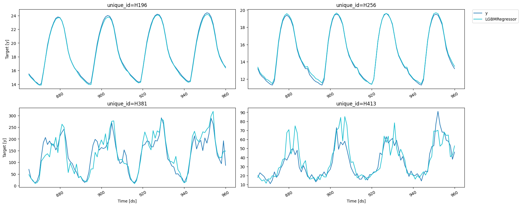
```python theme={null}
fig = plot_series(forecasts_df=cv_results.drop(columns='cutoff'))
fig
```
### Preprocess
If you want to take a look at the data that will be used to train the
models you can call `Forecast.preprocess`.
```python theme={null}
prep_df = fcst.preprocess(train)
prep_df
```
| | unique\_id | ds | y | lag24 | lag48 | lag72 | lag96 | lag120 | lag144 | lag168 | exponentially\_weighted\_mean\_lag48\_alpha0.3 |
| ------ | ---------- | --- | ---- | ----- | ----- | ----- | ----- | ------ | ------ | ------ | ---------------------------------------------- |
| 86988 | H196 | 193 | 0.1 | 0.0 | 0.0 | 0.0 | 0.3 | 0.1 | 0.1 | 0.3 | 0.002810 |
| 86989 | H196 | 194 | 0.1 | -0.1 | 0.1 | 0.0 | 0.3 | 0.1 | 0.1 | 0.3 | 0.031967 |
| 86990 | H196 | 195 | 0.1 | -0.1 | 0.1 | 0.0 | 0.3 | 0.1 | 0.2 | 0.1 | 0.052377 |
| 86991 | H196 | 196 | 0.1 | 0.0 | 0.0 | 0.0 | 0.3 | 0.2 | 0.1 | 0.2 | 0.036664 |
| 86992 | H196 | 197 | 0.0 | 0.0 | 0.0 | 0.1 | 0.2 | 0.2 | 0.1 | 0.2 | 0.025665 |
| ... | ... | ... | ... | ... | ... | ... | ... | ... | ... | ... | ... |
| 325187 | H413 | 956 | 0.0 | 10.0 | 1.0 | 6.0 | -53.0 | 44.0 | -21.0 | 21.0 | 7.963225 |
| 325188 | H413 | 957 | 9.0 | 10.0 | 10.0 | -7.0 | -46.0 | 27.0 | -19.0 | 24.0 | 8.574257 |
| 325189 | H413 | 958 | 16.0 | 8.0 | 5.0 | -9.0 | -36.0 | 32.0 | -13.0 | 8.0 | 7.501980 |
| 325190 | H413 | 959 | -3.0 | 17.0 | -7.0 | 2.0 | -31.0 | 22.0 | 5.0 | -2.0 | 3.151386 |
| 325191 | H413 | 960 | 15.0 | 11.0 | -6.0 | -5.0 | -17.0 | 22.0 | -18.0 | 10.0 | 0.405970 |
If we do this we then have to call `Forecast.fit_models`, since this
only stores the series information.
```python theme={null}
X, y = prep_df.drop(columns=['unique_id', 'ds', 'y']), prep_df['y']
fcst.fit_models(X, y)
```
```text theme={null}
MLForecast(models=[LGBMRegressor], freq=1, lag_features=['lag24', 'lag48', 'lag72', 'lag96', 'lag120', 'lag144', 'lag168', 'exponentially_weighted_mean_lag48_alpha0.3'], date_features=[], num_threads=1)
```
```python theme={null}
fcst
```
```text theme={null}
MLForecast(models=[LGBMRegressor], freq=1, lag_features=['lag24', 'lag48', 'lag72', 'lag96', 'lag120', 'lag144', 'lag168', 'exponentially_weighted_mean_lag48_alpha0.3'], date_features=[], num_threads=1)
```
```python theme={null}
predictions2 = fcst.predict(horizon)
pd.testing.assert_frame_equal(predictions, predictions2)
```
If we would like to know how good our forecast will be for a specific
model and set of features then we can perform cross validation. What
cross validation does is take our data and split it in two parts, where
the first part is used for training and the second one for validation.
Since the data is time dependant we usually take the last *x*
observations from our data as the validation set.
This process is implemented in
[`MLForecast.cross_validation`](https://Nixtla.github.io/mlforecast/forecast.html#mlforecast.cross_validation),
which takes our data and performs the process described above for
`n_windows` times where each window has `h` validation samples in it.
For example, if we have 100 samples and we want to perform 2 backtests
each of size 14, the splits will be as follows:
1. Train: 1 to 72. Validation: 73 to 86.
2. Train: 1 to 86. Validation: 87 to 100.
You can control the size between each cross validation window using the
`step_size` argument. For example, if we have 100 samples and we want to
perform 2 backtests each of size 14 and move one step ahead in each fold
(`step_size=1`), the splits will be as follows:
1. Train: 1 to 85. Validation: 86 to 99.
2. Train: 1 to 86. Validation: 87 to 100.
You can also perform cross validation without refitting your models for
each window by setting `refit=False`. This allows you to evaluate the
performance of your models using multiple window sizes without having to
retrain them each time.
```python theme={null}
fcst = MLForecast(
models=lgb.LGBMRegressor(random_state=0, verbosity=-1),
freq=1,
lags=[24 * (i+1) for i in range(7)],
lag_transforms={
1: [RollingMean(window_size=24)],
24: [RollingMean(window_size=24)],
48: [ExponentiallyWeightedMean(alpha=0.3)],
},
num_threads=1,
target_transforms=[Differences([24])],
)
cv_results = fcst.cross_validation(
train,
n_windows=2,
h=horizon,
step_size=horizon,
fitted=True,
)
cv_results
```
| | unique\_id | ds | cutoff | y | LGBMRegressor |
| --- | ---------- | --- | ------ | ---- | ------------- |
| 0 | H196 | 865 | 864 | 15.5 | 15.373393 |
| 1 | H196 | 866 | 864 | 15.1 | 14.973393 |
| 2 | H196 | 867 | 864 | 14.8 | 14.673393 |
| 3 | H196 | 868 | 864 | 14.4 | 14.373393 |
| 4 | H196 | 869 | 864 | 14.2 | 14.073393 |
| ... | ... | ... | ... | ... | ... |
| 379 | H413 | 956 | 912 | 59.0 | 64.284167 |
| 380 | H413 | 957 | 912 | 58.0 | 64.830429 |
| 381 | H413 | 958 | 912 | 53.0 | 40.726851 |
| 382 | H413 | 959 | 912 | 38.0 | 42.739657 |
| 383 | H413 | 960 | 912 | 46.0 | 52.802769 |
Since we set `fitted=True` we can access the predictions for the
training sets as well with the `cross_validation_fitted_values` method.
```python theme={null}
fcst.cross_validation_fitted_values()
```
| | unique\_id | ds | fold | y | LGBMRegressor |
| ---- | ---------- | --- | ---- | ---- | ------------- |
| 0 | H196 | 193 | 0 | 12.7 | 12.673393 |
| 1 | H196 | 194 | 0 | 12.3 | 12.273393 |
| 2 | H196 | 195 | 0 | 11.9 | 11.873393 |
| 3 | H196 | 196 | 0 | 11.7 | 11.673393 |
| 4 | H196 | 197 | 0 | 11.4 | 11.473393 |
| ... | ... | ... | ... | ... | ... |
| 5563 | H413 | 908 | 1 | 49.0 | 50.620196 |
| 5564 | H413 | 909 | 1 | 39.0 | 35.972331 |
| 5565 | H413 | 910 | 1 | 29.0 | 29.359678 |
| 5566 | H413 | 911 | 1 | 24.0 | 25.784563 |
| 5567 | H413 | 912 | 1 | 20.0 | 23.168413 |
We can also compute prediction intervals by passing a configuration to
`prediction_intervals` as well as values for the width through `levels`.
```python theme={null}
cv_results_intervals = fcst.cross_validation(
train,
n_windows=2,
h=horizon,
step_size=horizon,
prediction_intervals=PredictionIntervals(h=horizon),
level=[80, 90]
)
cv_results_intervals
```
| | unique\_id | ds | cutoff | y | LGBMRegressor | LGBMRegressor-lo-90 | LGBMRegressor-lo-80 | LGBMRegressor-hi-80 | LGBMRegressor-hi-90 |
| --- | ---------- | --- | ------ | ---- | ------------- | ------------------- | ------------------- | ------------------- | ------------------- |
| 0 | H196 | 865 | 864 | 15.5 | 15.373393 | 15.311379 | 15.316528 | 15.430258 | 15.435407 |
| 1 | H196 | 866 | 864 | 15.1 | 14.973393 | 14.940556 | 14.940556 | 15.006230 | 15.006230 |
| 2 | H196 | 867 | 864 | 14.8 | 14.673393 | 14.606230 | 14.606230 | 14.740556 | 14.740556 |
| 3 | H196 | 868 | 864 | 14.4 | 14.373393 | 14.306230 | 14.306230 | 14.440556 | 14.440556 |
| 4 | H196 | 869 | 864 | 14.2 | 14.073393 | 14.006230 | 14.006230 | 14.140556 | 14.140556 |
| ... | ... | ... | ... | ... | ... | ... | ... | ... | ... |
| 379 | H413 | 956 | 912 | 59.0 | 64.284167 | 29.890099 | 34.371545 | 94.196788 | 98.678234 |
| 380 | H413 | 957 | 912 | 58.0 | 64.830429 | 56.874572 | 57.827689 | 71.833169 | 72.786285 |
| 381 | H413 | 958 | 912 | 53.0 | 40.726851 | 35.296195 | 35.846206 | 45.607495 | 46.157506 |
| 382 | H413 | 959 | 912 | 38.0 | 42.739657 | 35.292153 | 35.807640 | 49.671674 | 50.187161 |
| 383 | H413 | 960 | 912 | 46.0 | 52.802769 | 42.465597 | 43.895670 | 61.709869 | 63.139941 |
The `refit` argument allows us to control if we want to retrain the
models in every window. It can either be:
* A boolean: True will retrain on every window and False only on the
first one.
* A positive integer: The models will be trained on the first window
and then every `refit` windows.
```python theme={null}
fcst = MLForecast(
models=LinearRegression(),
freq=1,
lags=[1, 24],
)
for refit, expected_models in zip([True, False, 2], [4, 1, 2]):
fcst.cross_validation(
train,
n_windows=4,
h=horizon,
refit=refit,
)
assert len(fcst.cv_models_) == expected_models
```
```python theme={null}
fig = plot_series(forecasts_df=cv_results.drop(columns='cutoff'))
fig
```
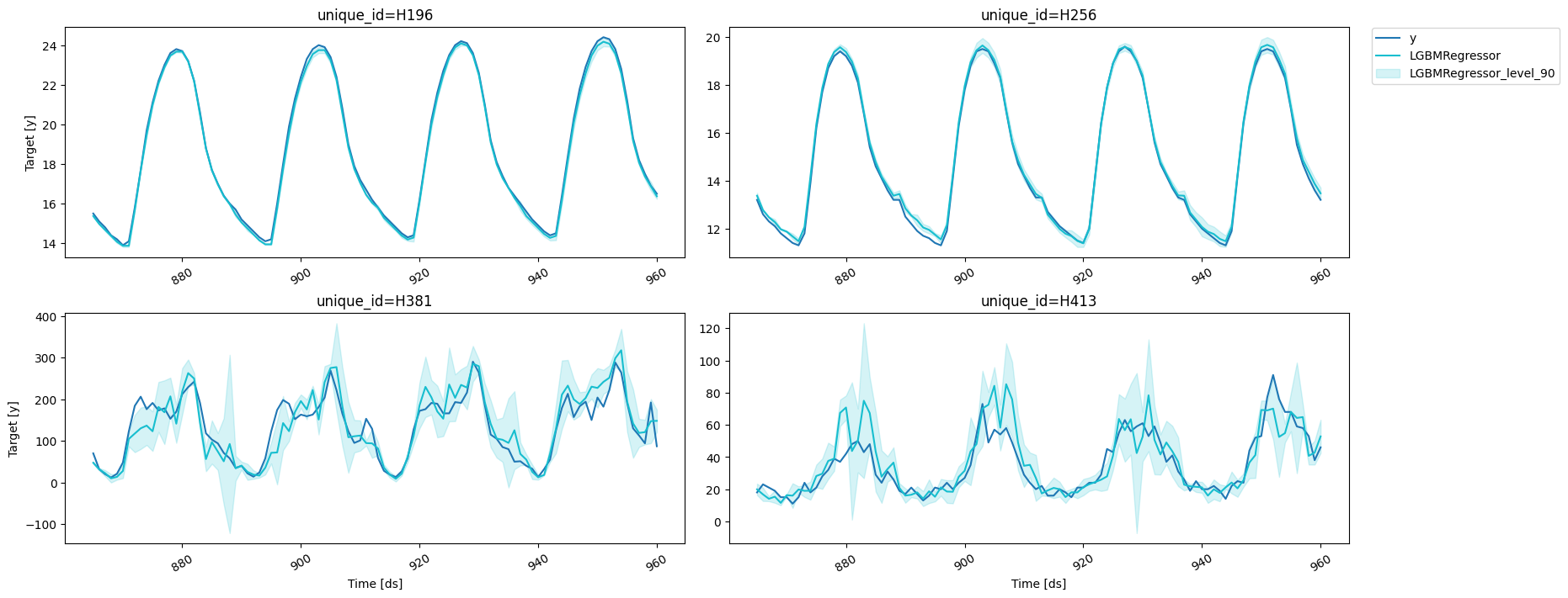
 ```python theme={null}
fig = plot_series(forecasts_df=cv_results_intervals.drop(columns='cutoff'), level=[90])
fig
```
```python theme={null}
fig = plot_series(forecasts_df=cv_results_intervals.drop(columns='cutoff'), level=[90])
fig
```
 ### Using LightGBMCV to tune your forecasts
Once you’ve found a set of features and parameters that work for your
problem you can build a forecast object from it using
[`MLForecast.from_cv`](https://Nixtla.github.io/mlforecast/forecast.html#mlforecast.from_cv),
which takes the trained
[`LightGBMCV`](https://Nixtla.github.io/mlforecast/lgb_cv.html#lightgbmcv)
object and builds an
[`MLForecast`](https://Nixtla.github.io/mlforecast/forecast.html#mlforecast)
object that will use the same features and parameters. Then you can call
fit and predict as you normally would.
```python theme={null}
cv = LightGBMCV(
freq=1,
lags=[24 * (i+1) for i in range(7)],
lag_transforms={
48: [ExponentiallyWeightedMean(alpha=0.3)],
},
num_threads=1,
target_transforms=[Differences([24])]
)
hist = cv.fit(
train,
n_windows=2,
h=horizon,
params={'verbosity': -1},
)
```
```text theme={null}
[10] mape: 0.118569
[20] mape: 0.111506
[30] mape: 0.107314
[40] mape: 0.106089
[50] mape: 0.106630
Early stopping at round 50
Using best iteration: 40
```
```python theme={null}
fcst = MLForecast.from_cv(cv)
assert cv.best_iteration_ == fcst.models['LGBMRegressor'].n_estimators
```
### Using LightGBMCV to tune your forecasts
Once you’ve found a set of features and parameters that work for your
problem you can build a forecast object from it using
[`MLForecast.from_cv`](https://Nixtla.github.io/mlforecast/forecast.html#mlforecast.from_cv),
which takes the trained
[`LightGBMCV`](https://Nixtla.github.io/mlforecast/lgb_cv.html#lightgbmcv)
object and builds an
[`MLForecast`](https://Nixtla.github.io/mlforecast/forecast.html#mlforecast)
object that will use the same features and parameters. Then you can call
fit and predict as you normally would.
```python theme={null}
cv = LightGBMCV(
freq=1,
lags=[24 * (i+1) for i in range(7)],
lag_transforms={
48: [ExponentiallyWeightedMean(alpha=0.3)],
},
num_threads=1,
target_transforms=[Differences([24])]
)
hist = cv.fit(
train,
n_windows=2,
h=horizon,
params={'verbosity': -1},
)
```
```text theme={null}
[10] mape: 0.118569
[20] mape: 0.111506
[30] mape: 0.107314
[40] mape: 0.106089
[50] mape: 0.106630
Early stopping at round 50
Using best iteration: 40
```
```python theme={null}
fcst = MLForecast.from_cv(cv)
assert cv.best_iteration_ == fcst.models['LGBMRegressor'].n_estimators
```