> ## Documentation Index
> Fetch the complete documentation index at: https://nixtlaverse.nixtla.io/llms.txt
> Use this file to discover all available pages before exploring further.
# Electricity Load Forecast | MLForecast
> In this example we will show how to perform electricity load
> forecasting using MLForecast alongside many models. We also compare
> them against the prophet library.
## Introduction
Some time series are generated from very low frequency data. These data
generally exhibit multiple seasonalities. For example, hourly data may
exhibit repeated patterns every hour (every 24 observations) or every
day (every 24 \* 7, hours per day, observations). This is the case for
electricity load. Electricity load may vary hourly, e.g., during the
evenings electricity consumption may be expected to increase. But also,
the electricity load varies by week. Perhaps on weekends there is an
increase in electrical activity.
In this example we will show how to model the two seasonalities of the
time series to generate accurate forecasts in a short time. We will use
hourly PJM electricity load data. The original data can be found
[here](https://www.kaggle.com/datasets/robikscube/hourly-energy-consumption).
## Libraries
In this example we will use the following libraries:
* [`mlforecast`](https://nixtlaverse.nixtla.io/mlforecast/). Accurate
and ⚡️ fast forecasting with classical machine learning models.
* [`prophet`](https://github.com/facebook/prophet). Benchmark model
developed by Facebook.
* [`utilsforecast`](https://nixtlaverse.nixtla.io/utilsforecast/).
Library with different functions for forecasting evaluation.
If you have already installed the libraries you can skip the next cell,
if not be sure to run it.
```python theme={null}
# %%capture
# !pip install prophet
# !pip install -U mlforecast
# !pip install -U utilsforecast
```
## Forecast using Multiple Seasonalities
### Electricity Load Data
According to the [dataset’s
page](https://www.kaggle.com/datasets/robikscube/hourly-energy-consumption),
> PJM Interconnection LLC (PJM) is a regional transmission organization
> (RTO) in the United States. It is part of the Eastern Interconnection
> grid operating an electric transmission system serving all or parts of
> Delaware, Illinois, Indiana, Kentucky, Maryland, Michigan, New Jersey,
> North Carolina, Ohio, Pennsylvania, Tennessee, Virginia, West
> Virginia, and the District of Columbia. The hourly power consumption
> data comes from PJM’s website and are in megawatts (MW).
Let’s take a look to the data.
```python theme={null}
import matplotlib.pyplot as plt
import numpy as np
import pandas as pd
from utilsforecast.plotting import plot_series
```
```python theme={null}
pd.plotting.register_matplotlib_converters()
plt.rc("figure", figsize=(10, 8))
plt.rc("font", size=10)
```
```python theme={null}
data_url = 'https://raw.githubusercontent.com/panambY/Hourly_Energy_Consumption/master/data/PJM_Load_hourly.csv'
df = pd.read_csv(data_url, parse_dates=['Datetime'])
df.columns = ['ds', 'y']
df.insert(0, 'unique_id', 'PJM_Load_hourly')
df['ds'] = pd.to_datetime(df['ds'])
df = df.sort_values(['unique_id', 'ds']).reset_index(drop=True)
print(f'Shape of the data {df.shape}')
df.tail()
```
```text theme={null}
Shape of the data (32896, 3)
```
| | unique\_id | ds | y |
| ----- | ----------------- | ------------------- | ------- |
| 32891 | PJM\_Load\_hourly | 2001-12-31 20:00:00 | 36392.0 |
| 32892 | PJM\_Load\_hourly | 2001-12-31 21:00:00 | 35082.0 |
| 32893 | PJM\_Load\_hourly | 2001-12-31 22:00:00 | 33890.0 |
| 32894 | PJM\_Load\_hourly | 2001-12-31 23:00:00 | 32590.0 |
| 32895 | PJM\_Load\_hourly | 2002-01-01 00:00:00 | 31569.0 |
```python theme={null}
fig = plot_series(df)
```
 We clearly observe that the time series exhibits seasonal patterns.
Moreover, the time series contains `32,896` observations, so it is
necessary to use very computationally efficient methods to display them
in production.
We are going to split our series in order to create a train and test
set. The model will be tested using the last 24 hours of the timeseries.
```python theme={null}
threshold_time = df['ds'].max() - pd.Timedelta(hours=24)
# Split the dataframe
df_train = df[df['ds'] <= threshold_time]
df_last_24_hours = df[df['ds'] > threshold_time]
```
### Analizing Seasonalities
First we must visualize the seasonalities of the model. As mentioned
before, the electricity load presents seasonalities every 24 hours
(Hourly) and every 24 \* 7 (Daily) hours. Therefore, we will use
`[24, 24 * 7]` as the seasonalities for the model. In order to analize
how they affect our series we are going to use the `Difference` method.
```python theme={null}
from mlforecast import MLForecast
from mlforecast.target_transforms import Differences
```
We can use the `MLForecast.preprocess` method to explore different
transformations. It looks like these series have a strong seasonality on
the hour of the day, so we can subtract the value from the same hour in
the previous day to remove it. This can be done with the
`mlforecast.target_transforms.Differences` transformer, which we pass
through `target_transforms`.
In order to analize the trends individually and combined we are going to
plot them individually and combined. Therefore, we can compare them
against the original series. We can use the next function for that.
```python theme={null}
def plot_differences(df, differences,fname):
prep = [df]
# Plot individual Differences
for d in differences:
fcst = MLForecast(
models=[], # we're not interested in modeling yet
freq='H', # our series have hourly frequency
target_transforms=[Differences([d])],
)
df_ = fcst.preprocess(df)
df_['unique_id'] = df_['unique_id'] + f'_{d}'
prep.append(df_)
# Plot combined Differences
fcst = MLForecast(
models=[], # we're not interested in modeling yet
freq='H', # our series have hourly frequency
target_transforms=[Differences([24, 24*7])],
)
df_ = fcst.preprocess(df)
df_['unique_id'] = df_['unique_id'] + f'_all_diff'
prep.append(df_)
prep = pd.concat(prep, ignore_index=True)
#return prep
n_series = len(prep['unique_id'].unique())
fig, ax = plt.subplots(nrows=n_series, figsize=(7 * n_series, 10*n_series), squeeze=False)
for title, axi in zip(prep['unique_id'].unique(), ax.flat):
df_ = prep[prep['unique_id'] == title]
df_.set_index('ds')['y'].plot(title=title, ax=axi)
fig.savefig(f'../../figs/{fname}', bbox_inches='tight')
plt.close()
```
Since the seasonalities are present at `24` hours (daily) and `24*7`
(weekly) we are going to subtract them from the serie using
`Differences([24, 24*7])` and plot them.
```python theme={null}
plot_differences(df=df_train, differences=[24, 24*7], fname='load_forecasting__differences.png')
```
We clearly observe that the time series exhibits seasonal patterns.
Moreover, the time series contains `32,896` observations, so it is
necessary to use very computationally efficient methods to display them
in production.
We are going to split our series in order to create a train and test
set. The model will be tested using the last 24 hours of the timeseries.
```python theme={null}
threshold_time = df['ds'].max() - pd.Timedelta(hours=24)
# Split the dataframe
df_train = df[df['ds'] <= threshold_time]
df_last_24_hours = df[df['ds'] > threshold_time]
```
### Analizing Seasonalities
First we must visualize the seasonalities of the model. As mentioned
before, the electricity load presents seasonalities every 24 hours
(Hourly) and every 24 \* 7 (Daily) hours. Therefore, we will use
`[24, 24 * 7]` as the seasonalities for the model. In order to analize
how they affect our series we are going to use the `Difference` method.
```python theme={null}
from mlforecast import MLForecast
from mlforecast.target_transforms import Differences
```
We can use the `MLForecast.preprocess` method to explore different
transformations. It looks like these series have a strong seasonality on
the hour of the day, so we can subtract the value from the same hour in
the previous day to remove it. This can be done with the
`mlforecast.target_transforms.Differences` transformer, which we pass
through `target_transforms`.
In order to analize the trends individually and combined we are going to
plot them individually and combined. Therefore, we can compare them
against the original series. We can use the next function for that.
```python theme={null}
def plot_differences(df, differences,fname):
prep = [df]
# Plot individual Differences
for d in differences:
fcst = MLForecast(
models=[], # we're not interested in modeling yet
freq='H', # our series have hourly frequency
target_transforms=[Differences([d])],
)
df_ = fcst.preprocess(df)
df_['unique_id'] = df_['unique_id'] + f'_{d}'
prep.append(df_)
# Plot combined Differences
fcst = MLForecast(
models=[], # we're not interested in modeling yet
freq='H', # our series have hourly frequency
target_transforms=[Differences([24, 24*7])],
)
df_ = fcst.preprocess(df)
df_['unique_id'] = df_['unique_id'] + f'_all_diff'
prep.append(df_)
prep = pd.concat(prep, ignore_index=True)
#return prep
n_series = len(prep['unique_id'].unique())
fig, ax = plt.subplots(nrows=n_series, figsize=(7 * n_series, 10*n_series), squeeze=False)
for title, axi in zip(prep['unique_id'].unique(), ax.flat):
df_ = prep[prep['unique_id'] == title]
df_.set_index('ds')['y'].plot(title=title, ax=axi)
fig.savefig(f'../../figs/{fname}', bbox_inches='tight')
plt.close()
```
Since the seasonalities are present at `24` hours (daily) and `24*7`
(weekly) we are going to subtract them from the serie using
`Differences([24, 24*7])` and plot them.
```python theme={null}
plot_differences(df=df_train, differences=[24, 24*7], fname='load_forecasting__differences.png')
```
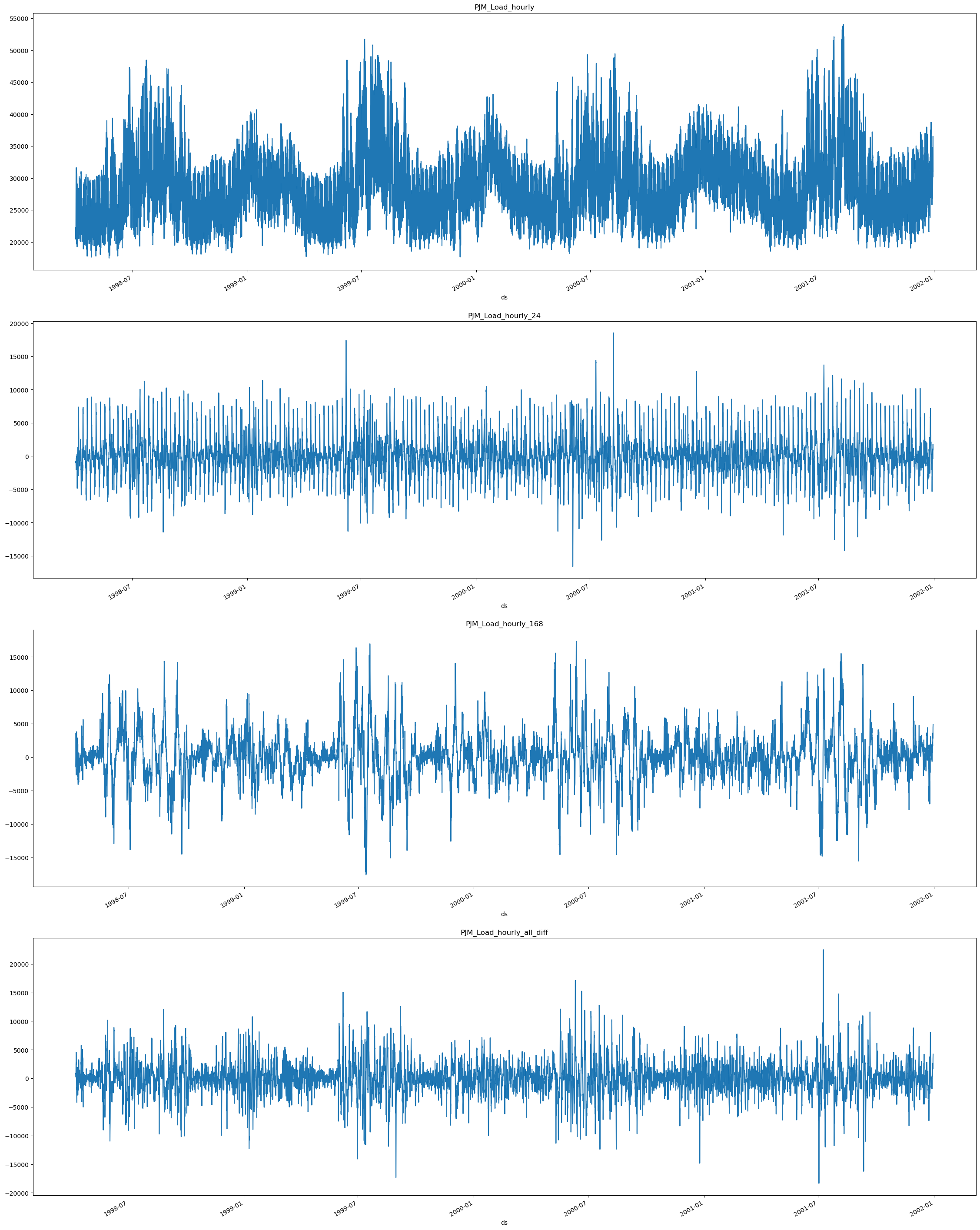 As we can see when we extract the 24 difference (daily) in
`PJM_Load_hourly_24` the series seem to stabilize since the peaks seem
more uniform in comparison with the original series `PJM_Load_hourly`.
When we extract the 24\*7 (weekly) `PJM_Load_hourly_168` difference we
can see there is more periodicity in the peaks in comparison with the
original series.
Finally we can see the result from the combined result from subtracting
all the differences `PJM_Load_hourly_all_diff`.
For modeling we are going to use both difference for the forecasting,
therefore we are setting the argument `target_transforms` from the
`MLForecast` object equal to `[Differences([24, 24*7])]`, if we wanted
to include a yearly difference we would need to add the term `24*365`.
```python theme={null}
fcst = MLForecast(
models=[], # we're not interested in modeling yet
freq='H', # our series have hourly frequency
target_transforms=[Differences([24, 24*7])],
)
prep = fcst.preprocess(df_train)
prep
```
| | unique\_id | ds | y |
| ----- | ----------------- | ------------------- | ------ |
| 192 | PJM\_Load\_hourly | 1998-04-09 02:00:00 | 831.0 |
| 193 | PJM\_Load\_hourly | 1998-04-09 03:00:00 | 918.0 |
| 194 | PJM\_Load\_hourly | 1998-04-09 04:00:00 | 760.0 |
| 195 | PJM\_Load\_hourly | 1998-04-09 05:00:00 | 849.0 |
| 196 | PJM\_Load\_hourly | 1998-04-09 06:00:00 | 710.0 |
| ... | ... | ... | ... |
| 32867 | PJM\_Load\_hourly | 2001-12-30 20:00:00 | 3417.0 |
| 32868 | PJM\_Load\_hourly | 2001-12-30 21:00:00 | 3596.0 |
| 32869 | PJM\_Load\_hourly | 2001-12-30 22:00:00 | 3501.0 |
| 32870 | PJM\_Load\_hourly | 2001-12-30 23:00:00 | 3939.0 |
| 32871 | PJM\_Load\_hourly | 2001-12-31 00:00:00 | 4235.0 |
```python theme={null}
fig = plot_series(prep)
```
As we can see when we extract the 24 difference (daily) in
`PJM_Load_hourly_24` the series seem to stabilize since the peaks seem
more uniform in comparison with the original series `PJM_Load_hourly`.
When we extract the 24\*7 (weekly) `PJM_Load_hourly_168` difference we
can see there is more periodicity in the peaks in comparison with the
original series.
Finally we can see the result from the combined result from subtracting
all the differences `PJM_Load_hourly_all_diff`.
For modeling we are going to use both difference for the forecasting,
therefore we are setting the argument `target_transforms` from the
`MLForecast` object equal to `[Differences([24, 24*7])]`, if we wanted
to include a yearly difference we would need to add the term `24*365`.
```python theme={null}
fcst = MLForecast(
models=[], # we're not interested in modeling yet
freq='H', # our series have hourly frequency
target_transforms=[Differences([24, 24*7])],
)
prep = fcst.preprocess(df_train)
prep
```
| | unique\_id | ds | y |
| ----- | ----------------- | ------------------- | ------ |
| 192 | PJM\_Load\_hourly | 1998-04-09 02:00:00 | 831.0 |
| 193 | PJM\_Load\_hourly | 1998-04-09 03:00:00 | 918.0 |
| 194 | PJM\_Load\_hourly | 1998-04-09 04:00:00 | 760.0 |
| 195 | PJM\_Load\_hourly | 1998-04-09 05:00:00 | 849.0 |
| 196 | PJM\_Load\_hourly | 1998-04-09 06:00:00 | 710.0 |
| ... | ... | ... | ... |
| 32867 | PJM\_Load\_hourly | 2001-12-30 20:00:00 | 3417.0 |
| 32868 | PJM\_Load\_hourly | 2001-12-30 21:00:00 | 3596.0 |
| 32869 | PJM\_Load\_hourly | 2001-12-30 22:00:00 | 3501.0 |
| 32870 | PJM\_Load\_hourly | 2001-12-30 23:00:00 | 3939.0 |
| 32871 | PJM\_Load\_hourly | 2001-12-31 00:00:00 | 4235.0 |
```python theme={null}
fig = plot_series(prep)
```
 ### Model Selection with Cross-Validation
We can test many models simultaneously using MLForecast
`cross_validation`. We can import `lightgbm` and `scikit-learn` models
and try different combinations of them, alongside different target
transformations (as the ones we created previously) and historical
variables.\
You can see an in-depth tutorial on how to use `MLForecast` [Cross
Validation methods
here](https://nixtlaverse.nixtla.io/mlforecast/docs/how-to-guides/cross_validation.html)
```python theme={null}
import lightgbm as lgb
from sklearn.base import BaseEstimator
from sklearn.linear_model import Lasso, LinearRegression, Ridge
from sklearn.neighbors import KNeighborsRegressor
from sklearn.neural_network import MLPRegressor
from sklearn.ensemble import RandomForestRegressor
from mlforecast.lag_transforms import ExpandingMean, RollingMean
from mlforecast.target_transforms import Differences
```
We can create a benchmark `Naive` model that uses the electricity load
of the last hour as prediction `lag1` as showed in the next cell. You
can create your own models and try them with `MLForecast` using the same
structure.
```python theme={null}
class Naive(BaseEstimator):
def fit(self, X, y):
return self
def predict(self, X):
return X['lag1']
```
Now let’s try differen models from the `scikit-learn` library: `Lasso`,
`LinearRegression`, `Ridge`, `KNN`, `MLP` and `Random Forest` alongside
the `LightGBM`. You can add any model to the dictionary to train and
compare them by adding them to the dictionary (`models`) as shown.
```python theme={null}
# Model dictionary
models ={
'naive': Naive(),
'lgbm': lgb.LGBMRegressor(verbosity=-1),
'lasso': Lasso(),
'lin_reg': LinearRegression(),
'ridge': Ridge(),
'knn': KNeighborsRegressor(),
'mlp': MLPRegressor(),
'rf': RandomForestRegressor()
}
```
The we can instanciate the `MLForecast` class with the models we want to
try along side `target_transforms`, `lags`, `lag_transforms`, and
`date_features`. All this features are applied to the models we
selected.
In this case we use the 1st, 12th and 24th lag, which are passed as a
list. Potentially you could pass a `range`.
```text theme={null}
lags=[1,12,24]
```
Lag transforms are defined as a dictionary where the keys are the lags
and the values are lists of the transformations that we want to apply to
that lag. You can refer to the [lag transformations
guide](../how-to-guides/lag_transforms_guide.html) for more details.
For using the date features you need to be sure that your time column is
made of timestamps. Then it might make sense to extract features like
week, dayofweek, quarter, etc. You can do that by passing a list of
strings with [pandas time/date
components](https://pandas.pydata.org/docs/user_guide/timeseries.html#time-date-components).
You can also pass functions that will take the time column as input, as
we’ll show here.\
Here we add month, hour and dayofweek features:
```text theme={null}
date_features=['month', 'hour', 'dayofweek']
```
```python theme={null}
mlf = MLForecast(
models = models,
freq='H', # our series have hourly frequency
target_transforms=[Differences([24, 24*7])],
lags=[1,12,24], # Lags to be used as features
lag_transforms={
1: [ExpandingMean()],
24: [RollingMean(window_size=48)],
},
date_features=['month', 'hour', 'dayofweek']
)
```
Now we use the `cross_validation` method to train and evalaute the
models. + `df`: Receives the training data + `h`: Forecast horizon +
`n_windows`: The number of folds we want to predict
You can specify the names of the time series id, time and target
columns. + `id_col`:Column that identifies each serie ( Default
*unique\_id* ) + `time_col`: Column that identifies each timestep, its
values can be timestamps or integer( Default *ds* ) +
`target_col`:Column that contains the target ( Default *y* )
```python theme={null}
crossvalidation_df = mlf.cross_validation(
df=df_train,
h=24,
n_windows=4,
refit=False,
)
crossvalidation_df.head()
```
| | unique\_id | ds | cutoff | y | naive | lgbm | lasso | lin\_reg | ridge | knn | mlp | rf |
| - | ----------------- | ------------------- | ---------- | ------- | ------- | ------------ | ------------ | ------------ | ------------ | ------- | ------------ | -------- |
| 0 | PJM\_Load\_hourly | 2001-12-27 01:00:00 | 2001-12-27 | 28332.0 | 28837.0 | 28526.505572 | 28703.185712 | 28702.625949 | 28702.625956 | 28479.0 | 28660.021947 | 27995.17 |
| 1 | PJM\_Load\_hourly | 2001-12-27 02:00:00 | 2001-12-27 | 27329.0 | 27969.0 | 27467.860847 | 27693.502318 | 27692.395954 | 27692.395969 | 27521.6 | 27584.635434 | 27112.50 |
| 2 | PJM\_Load\_hourly | 2001-12-27 03:00:00 | 2001-12-27 | 26986.0 | 27435.0 | 26605.710615 | 26991.795124 | 26990.157567 | 26990.157589 | 26451.6 | 26809.412477 | 26529.72 |
| 3 | PJM\_Load\_hourly | 2001-12-27 04:00:00 | 2001-12-27 | 27009.0 | 27401.0 | 26284.065138 | 26789.418399 | 26787.262262 | 26787.262291 | 26388.4 | 26523.416348 | 26490.83 |
| 4 | PJM\_Load\_hourly | 2001-12-27 05:00:00 | 2001-12-27 | 27555.0 | 28169.0 | 26823.617078 | 27369.643789 | 27366.983075 | 27366.983111 | 26779.6 | 26986.355992 | 27180.69 |
Now we can plot each model and window (fold) to see how it behaves
```python theme={null}
def plot_cv(df, df_cv, uid, fname, last_n=24 * 14, models={}):
cutoffs = df_cv.query('unique_id == @uid')['cutoff'].unique()
fig, ax = plt.subplots(nrows=len(cutoffs), ncols=1, figsize=(14, 14), gridspec_kw=dict(hspace=0.8))
for cutoff, axi in zip(cutoffs, ax.flat):
max_date = df_cv.query('unique_id == @uid & cutoff == @cutoff')['ds'].max()
df[df['ds'] < max_date].query('unique_id == @uid').tail(last_n).set_index('ds').plot(ax=axi, title=uid, y='y')
for m in models.keys():
df_cv.query('unique_id == @uid & cutoff == @cutoff').set_index('ds').plot(ax=axi, title=uid, y=m)
fig.savefig(f'../../figs/{fname}', bbox_inches='tight')
plt.close()
```
```python theme={null}
plot_cv(df_train, crossvalidation_df, 'PJM_Load_hourly', 'load_forecasting__predictions.png', models=models)
```
### Model Selection with Cross-Validation
We can test many models simultaneously using MLForecast
`cross_validation`. We can import `lightgbm` and `scikit-learn` models
and try different combinations of them, alongside different target
transformations (as the ones we created previously) and historical
variables.\
You can see an in-depth tutorial on how to use `MLForecast` [Cross
Validation methods
here](https://nixtlaverse.nixtla.io/mlforecast/docs/how-to-guides/cross_validation.html)
```python theme={null}
import lightgbm as lgb
from sklearn.base import BaseEstimator
from sklearn.linear_model import Lasso, LinearRegression, Ridge
from sklearn.neighbors import KNeighborsRegressor
from sklearn.neural_network import MLPRegressor
from sklearn.ensemble import RandomForestRegressor
from mlforecast.lag_transforms import ExpandingMean, RollingMean
from mlforecast.target_transforms import Differences
```
We can create a benchmark `Naive` model that uses the electricity load
of the last hour as prediction `lag1` as showed in the next cell. You
can create your own models and try them with `MLForecast` using the same
structure.
```python theme={null}
class Naive(BaseEstimator):
def fit(self, X, y):
return self
def predict(self, X):
return X['lag1']
```
Now let’s try differen models from the `scikit-learn` library: `Lasso`,
`LinearRegression`, `Ridge`, `KNN`, `MLP` and `Random Forest` alongside
the `LightGBM`. You can add any model to the dictionary to train and
compare them by adding them to the dictionary (`models`) as shown.
```python theme={null}
# Model dictionary
models ={
'naive': Naive(),
'lgbm': lgb.LGBMRegressor(verbosity=-1),
'lasso': Lasso(),
'lin_reg': LinearRegression(),
'ridge': Ridge(),
'knn': KNeighborsRegressor(),
'mlp': MLPRegressor(),
'rf': RandomForestRegressor()
}
```
The we can instanciate the `MLForecast` class with the models we want to
try along side `target_transforms`, `lags`, `lag_transforms`, and
`date_features`. All this features are applied to the models we
selected.
In this case we use the 1st, 12th and 24th lag, which are passed as a
list. Potentially you could pass a `range`.
```text theme={null}
lags=[1,12,24]
```
Lag transforms are defined as a dictionary where the keys are the lags
and the values are lists of the transformations that we want to apply to
that lag. You can refer to the [lag transformations
guide](../how-to-guides/lag_transforms_guide.html) for more details.
For using the date features you need to be sure that your time column is
made of timestamps. Then it might make sense to extract features like
week, dayofweek, quarter, etc. You can do that by passing a list of
strings with [pandas time/date
components](https://pandas.pydata.org/docs/user_guide/timeseries.html#time-date-components).
You can also pass functions that will take the time column as input, as
we’ll show here.\
Here we add month, hour and dayofweek features:
```text theme={null}
date_features=['month', 'hour', 'dayofweek']
```
```python theme={null}
mlf = MLForecast(
models = models,
freq='H', # our series have hourly frequency
target_transforms=[Differences([24, 24*7])],
lags=[1,12,24], # Lags to be used as features
lag_transforms={
1: [ExpandingMean()],
24: [RollingMean(window_size=48)],
},
date_features=['month', 'hour', 'dayofweek']
)
```
Now we use the `cross_validation` method to train and evalaute the
models. + `df`: Receives the training data + `h`: Forecast horizon +
`n_windows`: The number of folds we want to predict
You can specify the names of the time series id, time and target
columns. + `id_col`:Column that identifies each serie ( Default
*unique\_id* ) + `time_col`: Column that identifies each timestep, its
values can be timestamps or integer( Default *ds* ) +
`target_col`:Column that contains the target ( Default *y* )
```python theme={null}
crossvalidation_df = mlf.cross_validation(
df=df_train,
h=24,
n_windows=4,
refit=False,
)
crossvalidation_df.head()
```
| | unique\_id | ds | cutoff | y | naive | lgbm | lasso | lin\_reg | ridge | knn | mlp | rf |
| - | ----------------- | ------------------- | ---------- | ------- | ------- | ------------ | ------------ | ------------ | ------------ | ------- | ------------ | -------- |
| 0 | PJM\_Load\_hourly | 2001-12-27 01:00:00 | 2001-12-27 | 28332.0 | 28837.0 | 28526.505572 | 28703.185712 | 28702.625949 | 28702.625956 | 28479.0 | 28660.021947 | 27995.17 |
| 1 | PJM\_Load\_hourly | 2001-12-27 02:00:00 | 2001-12-27 | 27329.0 | 27969.0 | 27467.860847 | 27693.502318 | 27692.395954 | 27692.395969 | 27521.6 | 27584.635434 | 27112.50 |
| 2 | PJM\_Load\_hourly | 2001-12-27 03:00:00 | 2001-12-27 | 26986.0 | 27435.0 | 26605.710615 | 26991.795124 | 26990.157567 | 26990.157589 | 26451.6 | 26809.412477 | 26529.72 |
| 3 | PJM\_Load\_hourly | 2001-12-27 04:00:00 | 2001-12-27 | 27009.0 | 27401.0 | 26284.065138 | 26789.418399 | 26787.262262 | 26787.262291 | 26388.4 | 26523.416348 | 26490.83 |
| 4 | PJM\_Load\_hourly | 2001-12-27 05:00:00 | 2001-12-27 | 27555.0 | 28169.0 | 26823.617078 | 27369.643789 | 27366.983075 | 27366.983111 | 26779.6 | 26986.355992 | 27180.69 |
Now we can plot each model and window (fold) to see how it behaves
```python theme={null}
def plot_cv(df, df_cv, uid, fname, last_n=24 * 14, models={}):
cutoffs = df_cv.query('unique_id == @uid')['cutoff'].unique()
fig, ax = plt.subplots(nrows=len(cutoffs), ncols=1, figsize=(14, 14), gridspec_kw=dict(hspace=0.8))
for cutoff, axi in zip(cutoffs, ax.flat):
max_date = df_cv.query('unique_id == @uid & cutoff == @cutoff')['ds'].max()
df[df['ds'] < max_date].query('unique_id == @uid').tail(last_n).set_index('ds').plot(ax=axi, title=uid, y='y')
for m in models.keys():
df_cv.query('unique_id == @uid & cutoff == @cutoff').set_index('ds').plot(ax=axi, title=uid, y=m)
fig.savefig(f'../../figs/{fname}', bbox_inches='tight')
plt.close()
```
```python theme={null}
plot_cv(df_train, crossvalidation_df, 'PJM_Load_hourly', 'load_forecasting__predictions.png', models=models)
```
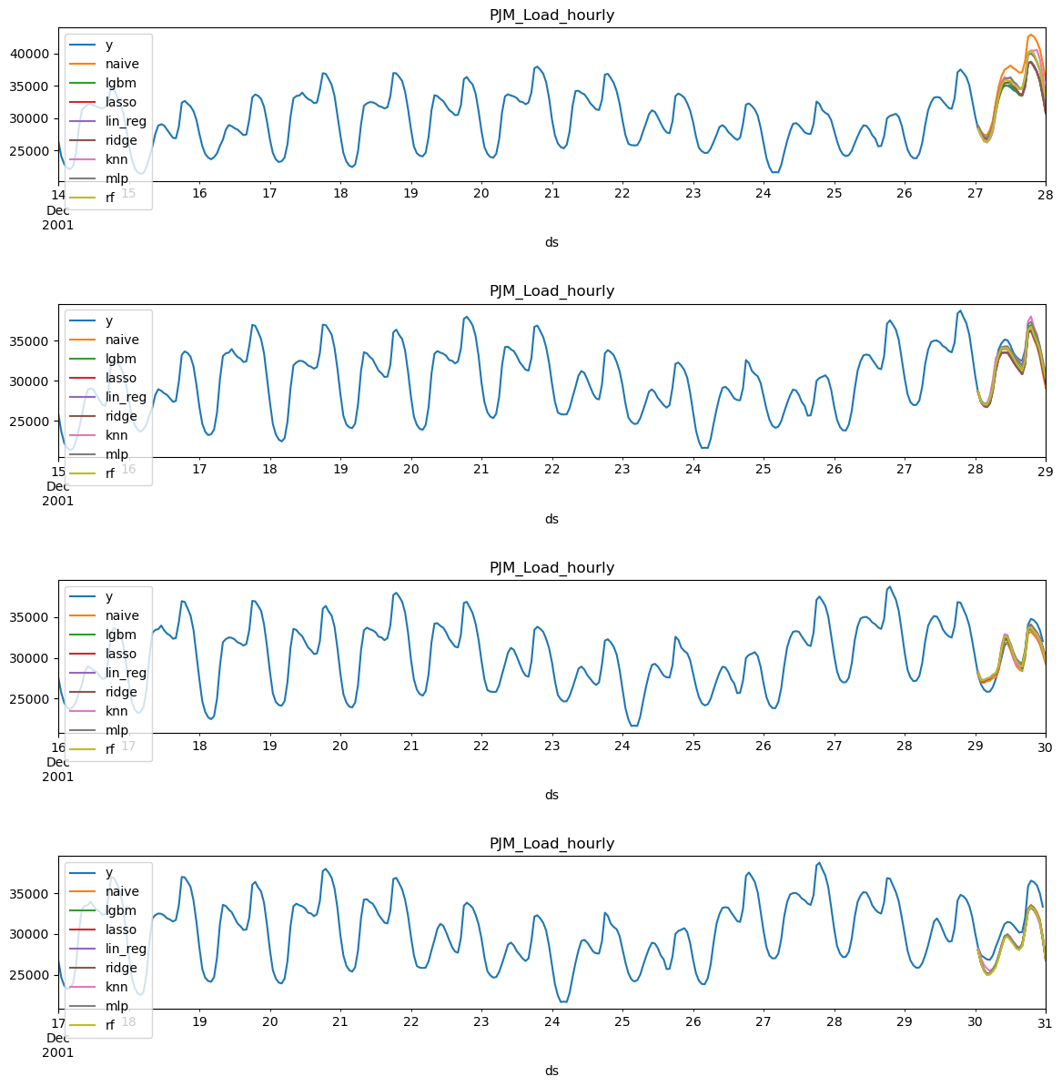 Visually examining the forecasts can give us some idea of how the model
is behaving, yet in order to asses the performace we need to evaluate
them trough metrics. For that we use the
[utilsforecast](https://nixtlaverse.nixtla.io/utilsforecast/) library
that contains many useful metrics and an evaluate function.
```python theme={null}
from utilsforecast.losses import mae, mape, rmse, smape
from utilsforecast.evaluation import evaluate
```
```python theme={null}
# Metrics to be used for evaluation
metrics = [
mae,
rmse,
mape,
smape
]
```
```python theme={null}
# Function to evaluate the crossvalidation
def evaluate_crossvalidation(crossvalidation_df, metrics, models):
evaluations = []
for c in crossvalidation_df['cutoff'].unique():
df_cv = crossvalidation_df.query('cutoff == @c')
evaluation = evaluate(
df = df_cv,
metrics=metrics,
models=list(models.keys())
)
evaluations.append(evaluation)
evaluations = pd.concat(evaluations, ignore_index=True).drop(columns='unique_id')
evaluations = evaluations.groupby('metric').mean()
return evaluations.style.background_gradient(cmap='RdYlGn_r', axis=1)
```
```python theme={null}
evaluate_crossvalidation(crossvalidation_df, metrics, models)
```
| | naive | lgbm | lasso | lin\_reg | ridge | knn | mlp | rf |
| ------ | ----------- | ----------- | ----------- | ----------- | ----------- | ----------- | ----------- | ----------- |
| metric | | | | | | | | |
| mae | 1631.395833 | 971.536200 | 1003.796433 | 1007.998597 | 1007.998547 | 1248.145833 | 1870.547722 | 1017.957813 |
| mape | 0.049759 | 0.030966 | 0.031760 | 0.031888 | 0.031888 | 0.038721 | 0.057504 | 0.032341 |
| rmse | 1871.398919 | 1129.713256 | 1148.616156 | 1153.262719 | 1153.262664 | 1451.964390 | 2102.098238 | 1154.647164 |
| smape | 0.024786 | 0.015886 | 0.016269 | 0.016338 | 0.016338 | 0.019549 | 0.029917 | 0.016563 |
We can see that the model `lgbm` has top performance in most metrics
followed by the `lasso regression`. Both models perform way better than
the `naive`.
### Test Evaluation
Now we are going to evaluate their performance in the test set. We can
use both of them for forecasting the test alongside some prediction
intervals. For that we can use the
[`PredictionIntervals`](https://nixtlaverse.nixtla.io/mlforecast/utils.html#predictionintervals)
function in `mlforecast.utils`.\
You can see an in-depth tutorial of [Probabilistic Forecasting
here](https://nixtlaverse.nixtla.io/mlforecast/docs/tutorials/prediction_intervals_in_forecasting_models)
```python theme={null}
from mlforecast.utils import PredictionIntervals
```
```python theme={null}
models_evaluation ={
'lgbm': lgb.LGBMRegressor(verbosity=-1),
'lasso': Lasso(),
}
mlf_evaluation = MLForecast(
models = models_evaluation,
freq='H', # our series have hourly frequency
target_transforms=[Differences([24, 24*7])],
lags=[1,12,24],
lag_transforms={
1: [ExpandingMean()],
24: [RollingMean(window_size=48)],
},
date_features=['month', 'hour', 'dayofweek']
)
```
Now we’re ready to generate the point forecasts and the prediction
intervals. To do this, we’ll use the `fit` method, which takes the
following arguments:
* `df`: Series data in long format.
* `id_col`: Column that identifies each series. In our case,
unique\_id.
* `time_col`: Column that identifies each timestep, its values can be
timestamps or integers. In our case, ds.
* `target_col`: Column that contains the target. In our case, y.
The `PredictionIntervals` function is used to compute prediction
intervals for the models using [Conformal
Prediction](https://valeman.medium.com/how-to-predict-full-probability-distribution-using-machine-learning-conformal-predictive-f8f4d805e420).
The function takes the following arguments: + `n_windows`: represents
the number of cross-validation windows used to calibrate the intervals +
`h`: the forecast horizon
```python theme={null}
mlf_evaluation.fit(
df = df_train,
prediction_intervals=PredictionIntervals(n_windows=4, h=24)
)
```
```text theme={null}
MLForecast(models=[lgbm, lasso], freq=H, lag_features=['lag1', 'lag12', 'lag24', 'expanding_mean_lag1', 'rolling_mean_lag24_window_size48'], date_features=['month', 'hour', 'dayofweek'], num_threads=1)
```
Now that the model has been trained we are going to forecast the next 24
hours using the `predict` method so we can compare them to our `test`
data. Additionally, we are going to create prediction intervals at
`levels` `[90,95]`.
```python theme={null}
levels = [90, 95] # Levels for prediction intervals
forecasts = mlf_evaluation.predict(24, level=levels)
forecasts.head()
```
| | unique\_id | ds | lgbm | lasso | lgbm-lo-95 | lgbm-lo-90 | lgbm-hi-90 | lgbm-hi-95 | lasso-lo-95 | lasso-lo-90 | lasso-hi-90 | lasso-hi-95 |
| - | ----------------- | ------------------- | ------------ | ------------ | ------------ | ------------ | ------------ | ------------ | ------------ | ------------ | ------------ | ------------ |
| 0 | PJM\_Load\_hourly | 2001-12-31 01:00:00 | 28847.573176 | 29124.085976 | 28544.593464 | 28567.603130 | 29127.543222 | 29150.552888 | 28762.752269 | 28772.604275 | 29475.567677 | 29485.419682 |
| 1 | PJM\_Load\_hourly | 2001-12-31 02:00:00 | 27862.589195 | 28365.330749 | 27042.311414 | 27128.839888 | 28596.338503 | 28682.866977 | 27528.548959 | 27619.065224 | 29111.596275 | 29202.112539 |
| 2 | PJM\_Load\_hourly | 2001-12-31 03:00:00 | 27044.418960 | 27712.161676 | 25596.659896 | 25688.230426 | 28400.607493 | 28492.178023 | 26236.955369 | 26338.087102 | 29086.236251 | 29187.367984 |
| 3 | PJM\_Load\_hourly | 2001-12-31 04:00:00 | 26976.104125 | 27661.572733 | 25249.961527 | 25286.024722 | 28666.183529 | 28702.246724 | 25911.133521 | 25959.815715 | 29363.329750 | 29412.011944 |
| 4 | PJM\_Load\_hourly | 2001-12-31 05:00:00 | 26694.246238 | 27393.922370 | 25044.220845 | 25051.548832 | 28336.943644 | 28344.271631 | 25751.547897 | 25762.524815 | 29025.319924 | 29036.296843 |
The `predict` method returns a DataFrame witht the predictions for each
model (`lasso` and `lgbm`) along side the prediction tresholds. The
high-threshold is indicated by the keyword `hi`, the low-threshold by
the keyword `lo`, and the level by the number in the column names.
```python theme={null}
test = df_last_24_hours.merge(forecasts, how='left', on=['unique_id', 'ds'])
test.head()
```
| | unique\_id | ds | y | lgbm | lasso | lgbm-lo-95 | lgbm-lo-90 | lgbm-hi-90 | lgbm-hi-95 | lasso-lo-95 | lasso-lo-90 | lasso-hi-90 | lasso-hi-95 |
| - | ----------------- | ------------------- | ------- | ------------ | ------------ | ------------ | ------------ | ------------ | ------------ | ------------ | ------------ | ------------ | ------------ |
| 0 | PJM\_Load\_hourly | 2001-12-31 01:00:00 | 29001.0 | 28847.573176 | 29124.085976 | 28544.593464 | 28567.603130 | 29127.543222 | 29150.552888 | 28762.752269 | 28772.604275 | 29475.567677 | 29485.419682 |
| 1 | PJM\_Load\_hourly | 2001-12-31 02:00:00 | 28138.0 | 27862.589195 | 28365.330749 | 27042.311414 | 27128.839888 | 28596.338503 | 28682.866977 | 27528.548959 | 27619.065224 | 29111.596275 | 29202.112539 |
| 2 | PJM\_Load\_hourly | 2001-12-31 03:00:00 | 27830.0 | 27044.418960 | 27712.161676 | 25596.659896 | 25688.230426 | 28400.607493 | 28492.178023 | 26236.955369 | 26338.087102 | 29086.236251 | 29187.367984 |
| 3 | PJM\_Load\_hourly | 2001-12-31 04:00:00 | 27874.0 | 26976.104125 | 27661.572733 | 25249.961527 | 25286.024722 | 28666.183529 | 28702.246724 | 25911.133521 | 25959.815715 | 29363.329750 | 29412.011944 |
| 4 | PJM\_Load\_hourly | 2001-12-31 05:00:00 | 28427.0 | 26694.246238 | 27393.922370 | 25044.220845 | 25051.548832 | 28336.943644 | 28344.271631 | 25751.547897 | 25762.524815 | 29025.319924 | 29036.296843 |
Now we can evaluate the metrics and performance in the `test` set.
```python theme={null}
evaluate(
df = test,
metrics=metrics,
models=list(models_evaluation.keys())
)
```
| | unique\_id | metric | lgbm | lasso |
| - | ----------------- | ------ | ----------- | ----------- |
| 0 | PJM\_Load\_hourly | mae | 1092.050817 | 899.979743 |
| 1 | PJM\_Load\_hourly | rmse | 1340.422762 | 1163.695525 |
| 2 | PJM\_Load\_hourly | mape | 0.033600 | 0.027688 |
| 3 | PJM\_Load\_hourly | smape | 0.017137 | 0.013812 |
We can see that the `lasso` regression performed slightly better than
the `LightGBM` for the test set. Additionally, we can also plot the
forecasts alongside their prediction intervals. For that we can use the
`plot_series` method available in `utilsforecast.plotting`.
We can plot one or many models at once alongside their confidence
intervals.
```python theme={null}
fig = plot_series(
df_train,
test,
models=['lasso', 'lgbm'],
plot_random=False,
level=levels,
max_insample_length=24
)
```
Visually examining the forecasts can give us some idea of how the model
is behaving, yet in order to asses the performace we need to evaluate
them trough metrics. For that we use the
[utilsforecast](https://nixtlaverse.nixtla.io/utilsforecast/) library
that contains many useful metrics and an evaluate function.
```python theme={null}
from utilsforecast.losses import mae, mape, rmse, smape
from utilsforecast.evaluation import evaluate
```
```python theme={null}
# Metrics to be used for evaluation
metrics = [
mae,
rmse,
mape,
smape
]
```
```python theme={null}
# Function to evaluate the crossvalidation
def evaluate_crossvalidation(crossvalidation_df, metrics, models):
evaluations = []
for c in crossvalidation_df['cutoff'].unique():
df_cv = crossvalidation_df.query('cutoff == @c')
evaluation = evaluate(
df = df_cv,
metrics=metrics,
models=list(models.keys())
)
evaluations.append(evaluation)
evaluations = pd.concat(evaluations, ignore_index=True).drop(columns='unique_id')
evaluations = evaluations.groupby('metric').mean()
return evaluations.style.background_gradient(cmap='RdYlGn_r', axis=1)
```
```python theme={null}
evaluate_crossvalidation(crossvalidation_df, metrics, models)
```
| | naive | lgbm | lasso | lin\_reg | ridge | knn | mlp | rf |
| ------ | ----------- | ----------- | ----------- | ----------- | ----------- | ----------- | ----------- | ----------- |
| metric | | | | | | | | |
| mae | 1631.395833 | 971.536200 | 1003.796433 | 1007.998597 | 1007.998547 | 1248.145833 | 1870.547722 | 1017.957813 |
| mape | 0.049759 | 0.030966 | 0.031760 | 0.031888 | 0.031888 | 0.038721 | 0.057504 | 0.032341 |
| rmse | 1871.398919 | 1129.713256 | 1148.616156 | 1153.262719 | 1153.262664 | 1451.964390 | 2102.098238 | 1154.647164 |
| smape | 0.024786 | 0.015886 | 0.016269 | 0.016338 | 0.016338 | 0.019549 | 0.029917 | 0.016563 |
We can see that the model `lgbm` has top performance in most metrics
followed by the `lasso regression`. Both models perform way better than
the `naive`.
### Test Evaluation
Now we are going to evaluate their performance in the test set. We can
use both of them for forecasting the test alongside some prediction
intervals. For that we can use the
[`PredictionIntervals`](https://nixtlaverse.nixtla.io/mlforecast/utils.html#predictionintervals)
function in `mlforecast.utils`.\
You can see an in-depth tutorial of [Probabilistic Forecasting
here](https://nixtlaverse.nixtla.io/mlforecast/docs/tutorials/prediction_intervals_in_forecasting_models)
```python theme={null}
from mlforecast.utils import PredictionIntervals
```
```python theme={null}
models_evaluation ={
'lgbm': lgb.LGBMRegressor(verbosity=-1),
'lasso': Lasso(),
}
mlf_evaluation = MLForecast(
models = models_evaluation,
freq='H', # our series have hourly frequency
target_transforms=[Differences([24, 24*7])],
lags=[1,12,24],
lag_transforms={
1: [ExpandingMean()],
24: [RollingMean(window_size=48)],
},
date_features=['month', 'hour', 'dayofweek']
)
```
Now we’re ready to generate the point forecasts and the prediction
intervals. To do this, we’ll use the `fit` method, which takes the
following arguments:
* `df`: Series data in long format.
* `id_col`: Column that identifies each series. In our case,
unique\_id.
* `time_col`: Column that identifies each timestep, its values can be
timestamps or integers. In our case, ds.
* `target_col`: Column that contains the target. In our case, y.
The `PredictionIntervals` function is used to compute prediction
intervals for the models using [Conformal
Prediction](https://valeman.medium.com/how-to-predict-full-probability-distribution-using-machine-learning-conformal-predictive-f8f4d805e420).
The function takes the following arguments: + `n_windows`: represents
the number of cross-validation windows used to calibrate the intervals +
`h`: the forecast horizon
```python theme={null}
mlf_evaluation.fit(
df = df_train,
prediction_intervals=PredictionIntervals(n_windows=4, h=24)
)
```
```text theme={null}
MLForecast(models=[lgbm, lasso], freq=H, lag_features=['lag1', 'lag12', 'lag24', 'expanding_mean_lag1', 'rolling_mean_lag24_window_size48'], date_features=['month', 'hour', 'dayofweek'], num_threads=1)
```
Now that the model has been trained we are going to forecast the next 24
hours using the `predict` method so we can compare them to our `test`
data. Additionally, we are going to create prediction intervals at
`levels` `[90,95]`.
```python theme={null}
levels = [90, 95] # Levels for prediction intervals
forecasts = mlf_evaluation.predict(24, level=levels)
forecasts.head()
```
| | unique\_id | ds | lgbm | lasso | lgbm-lo-95 | lgbm-lo-90 | lgbm-hi-90 | lgbm-hi-95 | lasso-lo-95 | lasso-lo-90 | lasso-hi-90 | lasso-hi-95 |
| - | ----------------- | ------------------- | ------------ | ------------ | ------------ | ------------ | ------------ | ------------ | ------------ | ------------ | ------------ | ------------ |
| 0 | PJM\_Load\_hourly | 2001-12-31 01:00:00 | 28847.573176 | 29124.085976 | 28544.593464 | 28567.603130 | 29127.543222 | 29150.552888 | 28762.752269 | 28772.604275 | 29475.567677 | 29485.419682 |
| 1 | PJM\_Load\_hourly | 2001-12-31 02:00:00 | 27862.589195 | 28365.330749 | 27042.311414 | 27128.839888 | 28596.338503 | 28682.866977 | 27528.548959 | 27619.065224 | 29111.596275 | 29202.112539 |
| 2 | PJM\_Load\_hourly | 2001-12-31 03:00:00 | 27044.418960 | 27712.161676 | 25596.659896 | 25688.230426 | 28400.607493 | 28492.178023 | 26236.955369 | 26338.087102 | 29086.236251 | 29187.367984 |
| 3 | PJM\_Load\_hourly | 2001-12-31 04:00:00 | 26976.104125 | 27661.572733 | 25249.961527 | 25286.024722 | 28666.183529 | 28702.246724 | 25911.133521 | 25959.815715 | 29363.329750 | 29412.011944 |
| 4 | PJM\_Load\_hourly | 2001-12-31 05:00:00 | 26694.246238 | 27393.922370 | 25044.220845 | 25051.548832 | 28336.943644 | 28344.271631 | 25751.547897 | 25762.524815 | 29025.319924 | 29036.296843 |
The `predict` method returns a DataFrame witht the predictions for each
model (`lasso` and `lgbm`) along side the prediction tresholds. The
high-threshold is indicated by the keyword `hi`, the low-threshold by
the keyword `lo`, and the level by the number in the column names.
```python theme={null}
test = df_last_24_hours.merge(forecasts, how='left', on=['unique_id', 'ds'])
test.head()
```
| | unique\_id | ds | y | lgbm | lasso | lgbm-lo-95 | lgbm-lo-90 | lgbm-hi-90 | lgbm-hi-95 | lasso-lo-95 | lasso-lo-90 | lasso-hi-90 | lasso-hi-95 |
| - | ----------------- | ------------------- | ------- | ------------ | ------------ | ------------ | ------------ | ------------ | ------------ | ------------ | ------------ | ------------ | ------------ |
| 0 | PJM\_Load\_hourly | 2001-12-31 01:00:00 | 29001.0 | 28847.573176 | 29124.085976 | 28544.593464 | 28567.603130 | 29127.543222 | 29150.552888 | 28762.752269 | 28772.604275 | 29475.567677 | 29485.419682 |
| 1 | PJM\_Load\_hourly | 2001-12-31 02:00:00 | 28138.0 | 27862.589195 | 28365.330749 | 27042.311414 | 27128.839888 | 28596.338503 | 28682.866977 | 27528.548959 | 27619.065224 | 29111.596275 | 29202.112539 |
| 2 | PJM\_Load\_hourly | 2001-12-31 03:00:00 | 27830.0 | 27044.418960 | 27712.161676 | 25596.659896 | 25688.230426 | 28400.607493 | 28492.178023 | 26236.955369 | 26338.087102 | 29086.236251 | 29187.367984 |
| 3 | PJM\_Load\_hourly | 2001-12-31 04:00:00 | 27874.0 | 26976.104125 | 27661.572733 | 25249.961527 | 25286.024722 | 28666.183529 | 28702.246724 | 25911.133521 | 25959.815715 | 29363.329750 | 29412.011944 |
| 4 | PJM\_Load\_hourly | 2001-12-31 05:00:00 | 28427.0 | 26694.246238 | 27393.922370 | 25044.220845 | 25051.548832 | 28336.943644 | 28344.271631 | 25751.547897 | 25762.524815 | 29025.319924 | 29036.296843 |
Now we can evaluate the metrics and performance in the `test` set.
```python theme={null}
evaluate(
df = test,
metrics=metrics,
models=list(models_evaluation.keys())
)
```
| | unique\_id | metric | lgbm | lasso |
| - | ----------------- | ------ | ----------- | ----------- |
| 0 | PJM\_Load\_hourly | mae | 1092.050817 | 899.979743 |
| 1 | PJM\_Load\_hourly | rmse | 1340.422762 | 1163.695525 |
| 2 | PJM\_Load\_hourly | mape | 0.033600 | 0.027688 |
| 3 | PJM\_Load\_hourly | smape | 0.017137 | 0.013812 |
We can see that the `lasso` regression performed slightly better than
the `LightGBM` for the test set. Additionally, we can also plot the
forecasts alongside their prediction intervals. For that we can use the
`plot_series` method available in `utilsforecast.plotting`.
We can plot one or many models at once alongside their confidence
intervals.
```python theme={null}
fig = plot_series(
df_train,
test,
models=['lasso', 'lgbm'],
plot_random=False,
level=levels,
max_insample_length=24
)
```
 ### Comparison with Prophet
One of the most widely used models for time series forecasting is
`Prophet`. This model is known for its ability to model different
seasonalities (weekly, daily yearly). We will use this model as a
benchmark to see if the `lgbm` alongside `MLForecast` adds value for
this time series.
```python theme={null}
from prophet import Prophet
from time import time
```
```text theme={null}
Importing plotly failed. Interactive plots will not work.
```
```python theme={null}
# create prophet model
prophet = Prophet(interval_width=0.9)
init = time()
prophet.fit(df_train)
# produce forecasts
future = prophet.make_future_dataframe(periods=len(df_last_24_hours), freq='H', include_history=False)
forecast_prophet = prophet.predict(future)
end = time()
# data wrangling
forecast_prophet = forecast_prophet[['ds', 'yhat', 'yhat_lower', 'yhat_upper']]
forecast_prophet.columns = ['ds', 'Prophet', 'Prophet-lo-90', 'Prophet-hi-90']
forecast_prophet.insert(0, 'unique_id', 'PJM_Load_hourly')
forecast_prophet.head()
```
| | unique\_id | ds | Prophet | Prophet-lo-90 | Prophet-hi-90 |
| - | ----------------- | ------------------- | ------------ | ------------- | ------------- |
| 0 | PJM\_Load\_hourly | 2001-12-31 01:00:00 | 25333.448442 | 20589.873559 | 30370.174820 |
| 1 | PJM\_Load\_hourly | 2001-12-31 02:00:00 | 24039.925936 | 18927.503487 | 29234.930903 |
| 2 | PJM\_Load\_hourly | 2001-12-31 03:00:00 | 23363.998793 | 18428.462513 | 28292.424622 |
| 3 | PJM\_Load\_hourly | 2001-12-31 04:00:00 | 23371.799609 | 18206.273446 | 28181.023448 |
| 4 | PJM\_Load\_hourly | 2001-12-31 05:00:00 | 24146.468610 | 19356.171497 | 29006.546759 |
```python theme={null}
time_prophet = (end - init)
print(f'Prophet Time: {time_prophet:.2f} seconds')
```
```text theme={null}
Prophet Time: 18.00 seconds
```
```python theme={null}
models_comparison ={
'lgbm': lgb.LGBMRegressor(verbosity=-1)
}
mlf_comparison = MLForecast(
models = models_comparison,
freq='H', # our series have hourly frequency
target_transforms=[Differences([24, 24*7])],
lags=[1,12,24],
lag_transforms={
1: [ExpandingMean()],
24: [RollingMean(window_size=48)],
},
date_features=['month', 'hour', 'dayofweek']
)
init = time()
mlf_comparison.fit(
df = df_train,
prediction_intervals=PredictionIntervals(n_windows=4, h=24)
)
levels = [90]
forecasts_comparison = mlf_comparison.predict(24, level=levels)
end = time()
forecasts_comparison.head()
```
| | unique\_id | ds | lgbm | lgbm-lo-90 | lgbm-hi-90 |
| - | ----------------- | ------------------- | ------------ | ------------ | ------------ |
| 0 | PJM\_Load\_hourly | 2001-12-31 01:00:00 | 28847.573176 | 28567.603130 | 29127.543222 |
| 1 | PJM\_Load\_hourly | 2001-12-31 02:00:00 | 27862.589195 | 27128.839888 | 28596.338503 |
| 2 | PJM\_Load\_hourly | 2001-12-31 03:00:00 | 27044.418960 | 25688.230426 | 28400.607493 |
| 3 | PJM\_Load\_hourly | 2001-12-31 04:00:00 | 26976.104125 | 25286.024722 | 28666.183529 |
| 4 | PJM\_Load\_hourly | 2001-12-31 05:00:00 | 26694.246238 | 25051.548832 | 28336.943644 |
```python theme={null}
time_lgbm = (end - init)
print(f'LGBM Time: {time_lgbm:.2f} seconds')
```
```text theme={null}
LGBM Time: 0.86 seconds
```
```python theme={null}
metrics_comparison = df_last_24_hours.merge(forecasts_comparison, how='left', on=['unique_id', 'ds']).merge(
forecast_prophet, how='left', on=['unique_id', 'ds'])
metrics_comparison = evaluate(
df = metrics_comparison,
metrics=metrics,
models=['Prophet', 'lgbm']
)
metrics_comparison.reset_index(drop=True).style.background_gradient(cmap='RdYlGn_r', axis=1)
```
| | unique\_id | metric | Prophet | lgbm |
| - | ----------------- | ------ | ----------- | ----------- |
| 0 | PJM\_Load\_hourly | mae | 2266.561642 | 1092.050817 |
| 1 | PJM\_Load\_hourly | rmse | 2701.302779 | 1340.422762 |
| 2 | PJM\_Load\_hourly | mape | 0.073226 | 0.033600 |
| 3 | PJM\_Load\_hourly | smape | 0.038320 | 0.017137 |
As we can see `lgbm` had consistently better metrics than `prophet`.
```python theme={null}
metrics_comparison['improvement'] = metrics_comparison['Prophet'] / metrics_comparison['lgbm']
metrics_comparison['improvement'] = metrics_comparison['improvement'].apply(lambda x: f'{x:.2f}')
metrics_comparison.set_index('metric')[['improvement']]
```
| | improvement |
| ------ | ----------- |
| metric | |
| mae | 2.08 |
| rmse | 2.02 |
| mape | 2.18 |
| smape | 2.24 |
```python theme={null}
print(f'lgbm with MLForecast has a speedup of {time_prophet/time_lgbm:.2f} compared with prophet')
```
```text theme={null}
lgbm with MLForecast has a speedup of 20.95 compared with prophet
```
We can see that `lgbm` with `MLForecast` was able to provide metrics at
least twice as good as `Prophet` as seen in the column `improvement`
above, and way faster.
### Comparison with Prophet
One of the most widely used models for time series forecasting is
`Prophet`. This model is known for its ability to model different
seasonalities (weekly, daily yearly). We will use this model as a
benchmark to see if the `lgbm` alongside `MLForecast` adds value for
this time series.
```python theme={null}
from prophet import Prophet
from time import time
```
```text theme={null}
Importing plotly failed. Interactive plots will not work.
```
```python theme={null}
# create prophet model
prophet = Prophet(interval_width=0.9)
init = time()
prophet.fit(df_train)
# produce forecasts
future = prophet.make_future_dataframe(periods=len(df_last_24_hours), freq='H', include_history=False)
forecast_prophet = prophet.predict(future)
end = time()
# data wrangling
forecast_prophet = forecast_prophet[['ds', 'yhat', 'yhat_lower', 'yhat_upper']]
forecast_prophet.columns = ['ds', 'Prophet', 'Prophet-lo-90', 'Prophet-hi-90']
forecast_prophet.insert(0, 'unique_id', 'PJM_Load_hourly')
forecast_prophet.head()
```
| | unique\_id | ds | Prophet | Prophet-lo-90 | Prophet-hi-90 |
| - | ----------------- | ------------------- | ------------ | ------------- | ------------- |
| 0 | PJM\_Load\_hourly | 2001-12-31 01:00:00 | 25333.448442 | 20589.873559 | 30370.174820 |
| 1 | PJM\_Load\_hourly | 2001-12-31 02:00:00 | 24039.925936 | 18927.503487 | 29234.930903 |
| 2 | PJM\_Load\_hourly | 2001-12-31 03:00:00 | 23363.998793 | 18428.462513 | 28292.424622 |
| 3 | PJM\_Load\_hourly | 2001-12-31 04:00:00 | 23371.799609 | 18206.273446 | 28181.023448 |
| 4 | PJM\_Load\_hourly | 2001-12-31 05:00:00 | 24146.468610 | 19356.171497 | 29006.546759 |
```python theme={null}
time_prophet = (end - init)
print(f'Prophet Time: {time_prophet:.2f} seconds')
```
```text theme={null}
Prophet Time: 18.00 seconds
```
```python theme={null}
models_comparison ={
'lgbm': lgb.LGBMRegressor(verbosity=-1)
}
mlf_comparison = MLForecast(
models = models_comparison,
freq='H', # our series have hourly frequency
target_transforms=[Differences([24, 24*7])],
lags=[1,12,24],
lag_transforms={
1: [ExpandingMean()],
24: [RollingMean(window_size=48)],
},
date_features=['month', 'hour', 'dayofweek']
)
init = time()
mlf_comparison.fit(
df = df_train,
prediction_intervals=PredictionIntervals(n_windows=4, h=24)
)
levels = [90]
forecasts_comparison = mlf_comparison.predict(24, level=levels)
end = time()
forecasts_comparison.head()
```
| | unique\_id | ds | lgbm | lgbm-lo-90 | lgbm-hi-90 |
| - | ----------------- | ------------------- | ------------ | ------------ | ------------ |
| 0 | PJM\_Load\_hourly | 2001-12-31 01:00:00 | 28847.573176 | 28567.603130 | 29127.543222 |
| 1 | PJM\_Load\_hourly | 2001-12-31 02:00:00 | 27862.589195 | 27128.839888 | 28596.338503 |
| 2 | PJM\_Load\_hourly | 2001-12-31 03:00:00 | 27044.418960 | 25688.230426 | 28400.607493 |
| 3 | PJM\_Load\_hourly | 2001-12-31 04:00:00 | 26976.104125 | 25286.024722 | 28666.183529 |
| 4 | PJM\_Load\_hourly | 2001-12-31 05:00:00 | 26694.246238 | 25051.548832 | 28336.943644 |
```python theme={null}
time_lgbm = (end - init)
print(f'LGBM Time: {time_lgbm:.2f} seconds')
```
```text theme={null}
LGBM Time: 0.86 seconds
```
```python theme={null}
metrics_comparison = df_last_24_hours.merge(forecasts_comparison, how='left', on=['unique_id', 'ds']).merge(
forecast_prophet, how='left', on=['unique_id', 'ds'])
metrics_comparison = evaluate(
df = metrics_comparison,
metrics=metrics,
models=['Prophet', 'lgbm']
)
metrics_comparison.reset_index(drop=True).style.background_gradient(cmap='RdYlGn_r', axis=1)
```
| | unique\_id | metric | Prophet | lgbm |
| - | ----------------- | ------ | ----------- | ----------- |
| 0 | PJM\_Load\_hourly | mae | 2266.561642 | 1092.050817 |
| 1 | PJM\_Load\_hourly | rmse | 2701.302779 | 1340.422762 |
| 2 | PJM\_Load\_hourly | mape | 0.073226 | 0.033600 |
| 3 | PJM\_Load\_hourly | smape | 0.038320 | 0.017137 |
As we can see `lgbm` had consistently better metrics than `prophet`.
```python theme={null}
metrics_comparison['improvement'] = metrics_comparison['Prophet'] / metrics_comparison['lgbm']
metrics_comparison['improvement'] = metrics_comparison['improvement'].apply(lambda x: f'{x:.2f}')
metrics_comparison.set_index('metric')[['improvement']]
```
| | improvement |
| ------ | ----------- |
| metric | |
| mae | 2.08 |
| rmse | 2.02 |
| mape | 2.18 |
| smape | 2.24 |
```python theme={null}
print(f'lgbm with MLForecast has a speedup of {time_prophet/time_lgbm:.2f} compared with prophet')
```
```text theme={null}
lgbm with MLForecast has a speedup of 20.95 compared with prophet
```
We can see that `lgbm` with `MLForecast` was able to provide metrics at
least twice as good as `Prophet` as seen in the column `improvement`
above, and way faster.