> ## Documentation Index
> Fetch the complete documentation index at: https://nixtlaverse.nixtla.io/llms.txt
> Use this file to discover all available pages before exploring further.
# Probabilistic forecasting | MLForecast
> In this example, we’ll implement prediction intervals
> **Prerequisites**
>
> This tutorial assumes basic familiarity with MLForecast. For a minimal
> example visit the [Quick
> Start](https://nixtlaverse.nixtla.io/mlforecast/docs/getting-started/quick_start_local.html)
## Introduction
When we generate a forecast, we usually produce a single value known as
the point forecast. This value, however, doesn’t tell us anything about
the uncertainty associated with the forecast. To have a measure of this
uncertainty, we need **prediction intervals**.
A prediction interval is a range of values that the forecast can take
with a given probability. Hence, a 95% prediction interval should
contain a range of values that include the actual future value with
probability 95%. Probabilistic forecasting aims to generate the full
forecast distribution. Point forecasting, on the other hand, usually
returns the mean or the median or said distribution. However, in
real-world scenarios, it is better to forecast not only the most
probable future outcome, but many alternative outcomes as well.
With [MLForecast](https://nixtla.github.io/mlforecast/) you can train
`sklearn` models to generate point forecasts. It also takes the
advantages of `ConformalPrediction` to generate the same point forecasts
and adds them prediction intervals. By the end of this tutorial, you’ll
have a good understanding of how to add probabilistic intervals to
`sklearn` models for time series forecasting. Furthermore, you’ll also
learn how to generate plots with the historical data, the point
forecasts, and the prediction intervals.
> **Important**
>
> Although the terms are often confused, prediction intervals are not
> the same as [confidence
> intervals](https://robjhyndman.com/hyndsight/intervals/).
> **Warning**
>
> In practice, most prediction intervals are too narrow since models do
> not account for all sources of uncertainty. A discussion about this
> can be found [here](https://robjhyndman.com/hyndsight/narrow-pi/).
**Outline:**
1. Install libraries
2. Load and explore the data
3. Train models
4. Plot prediction intervals
> **Tip**
>
> You can use Colab to run this Notebook interactively
>
>
>  >
## Install libraries
Install the necessary packages using
`pip install mlforecast utilsforecast`
## Load and explore the data
For this example, we’ll use the hourly dataset from the [M4
Competition](https://www.sciencedirect.com/science/article/pii/S0169207019301128).
We first need to download the data from a URL and then load it as a
`pandas` dataframe. Notice that we’ll load the train and the test data
separately. We’ll also rename the `y` column of the test data as
`y_test`.
```python theme={null}
import pandas as pd
from utilsforecast.plotting import plot_series
```
```python theme={null}
train = pd.read_csv('https://auto-arima-results.s3.amazonaws.com/M4-Hourly.csv')
test = pd.read_csv('https://auto-arima-results.s3.amazonaws.com/M4-Hourly-test.csv')
```
```python theme={null}
train.head()
```
| | unique\_id | ds | y |
| - | ---------- | -- | ----- |
| 0 | H1 | 1 | 605.0 |
| 1 | H1 | 2 | 586.0 |
| 2 | H1 | 3 | 586.0 |
| 3 | H1 | 4 | 559.0 |
| 4 | H1 | 5 | 511.0 |
```python theme={null}
test.head()
```
| | unique\_id | ds | y |
| - | ---------- | --- | ----- |
| 0 | H1 | 701 | 619.0 |
| 1 | H1 | 702 | 565.0 |
| 2 | H1 | 703 | 532.0 |
| 3 | H1 | 704 | 495.0 |
| 4 | H1 | 705 | 481.0 |
Since the goal of this notebook is to generate prediction intervals,
we’ll only use the first 8 series of the dataset to reduce the total
computational time.
```python theme={null}
n_series = 8
uids = train['unique_id'].unique()[:n_series] # select first n_series of the dataset
train = train.query('unique_id in @uids')
test = test.query('unique_id in @uids')
```
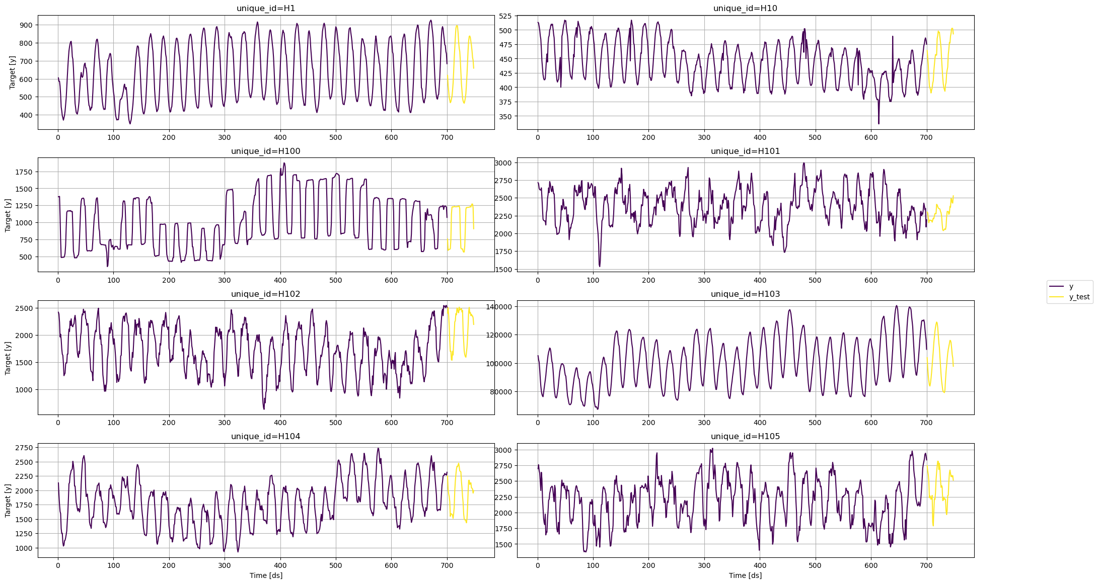
We can plot these series using the `plot_series` function from the
[utilsforecast](https://nixtla.github.io/utilsforecast/plotting.html)
library. This function has multiple parameters, and the required ones to
generate the plots in this notebook are explained below.
* `df`: A `pandas` dataframe with columns \[`unique_id`, `ds`, `y`].
* `forecasts_df`: A `pandas` dataframe with columns \[`unique_id`,
`ds`] and models.
* `plot_random`: bool = `True`. Plots the time series randomly.
* `models`: List\[str]. A list with the models we want to plot.
* `level`: List\[float]. A list with the prediction intervals we want
to plot.
* `engine`: str = `matplotlib`. It can also be `plotly`. `plotly`
generates interactive plots, while `matplotlib` generates static
plots.
```python theme={null}
fig = plot_series(train, test.rename(columns={'y': 'y_test'}), models=['y_test'], plot_random=False)
```
>
## Install libraries
Install the necessary packages using
`pip install mlforecast utilsforecast`
## Load and explore the data
For this example, we’ll use the hourly dataset from the [M4
Competition](https://www.sciencedirect.com/science/article/pii/S0169207019301128).
We first need to download the data from a URL and then load it as a
`pandas` dataframe. Notice that we’ll load the train and the test data
separately. We’ll also rename the `y` column of the test data as
`y_test`.
```python theme={null}
import pandas as pd
from utilsforecast.plotting import plot_series
```
```python theme={null}
train = pd.read_csv('https://auto-arima-results.s3.amazonaws.com/M4-Hourly.csv')
test = pd.read_csv('https://auto-arima-results.s3.amazonaws.com/M4-Hourly-test.csv')
```
```python theme={null}
train.head()
```
| | unique\_id | ds | y |
| - | ---------- | -- | ----- |
| 0 | H1 | 1 | 605.0 |
| 1 | H1 | 2 | 586.0 |
| 2 | H1 | 3 | 586.0 |
| 3 | H1 | 4 | 559.0 |
| 4 | H1 | 5 | 511.0 |
```python theme={null}
test.head()
```
| | unique\_id | ds | y |
| - | ---------- | --- | ----- |
| 0 | H1 | 701 | 619.0 |
| 1 | H1 | 702 | 565.0 |
| 2 | H1 | 703 | 532.0 |
| 3 | H1 | 704 | 495.0 |
| 4 | H1 | 705 | 481.0 |
Since the goal of this notebook is to generate prediction intervals,
we’ll only use the first 8 series of the dataset to reduce the total
computational time.
```python theme={null}
n_series = 8
uids = train['unique_id'].unique()[:n_series] # select first n_series of the dataset
train = train.query('unique_id in @uids')
test = test.query('unique_id in @uids')
```
We can plot these series using the `plot_series` function from the
[utilsforecast](https://nixtla.github.io/utilsforecast/plotting.html)
library. This function has multiple parameters, and the required ones to
generate the plots in this notebook are explained below.
* `df`: A `pandas` dataframe with columns \[`unique_id`, `ds`, `y`].
* `forecasts_df`: A `pandas` dataframe with columns \[`unique_id`,
`ds`] and models.
* `plot_random`: bool = `True`. Plots the time series randomly.
* `models`: List\[str]. A list with the models we want to plot.
* `level`: List\[float]. A list with the prediction intervals we want
to plot.
* `engine`: str = `matplotlib`. It can also be `plotly`. `plotly`
generates interactive plots, while `matplotlib` generates static
plots.
```python theme={null}
fig = plot_series(train, test.rename(columns={'y': 'y_test'}), models=['y_test'], plot_random=False)
```
 ## Train models
MLForecast can train multiple models that follow the `sklearn` syntax
(`fit` and `predict`) on different time series efficiently.
For this example, we’ll use the following `sklearn` baseline models:
* [Lasso](https://scikit-learn.org/stable/modules/generated/sklearn.linear_model.Lasso.html)
* [LinearRegression](https://scikit-learn.org/stable/modules/generated/sklearn.linear_model.LinearRegression.html)
* [Ridge](https://scikit-learn.org/stable/modules/generated/sklearn.linear_model.Ridge.html)
* [K-Nearest
Neighbors](https://scikit-learn.org/stable/modules/generated/sklearn.neighbors.KNeighborsRegressor.html)
* [Multilayer Perceptron
(NeuralNetwork)](https://scikit-learn.org/stable/modules/generated/sklearn.neural_network.MLPRegressor.html)
To use these models, we first need to import them from `sklearn` and
then we need to instantiate them.
```python theme={null}
from mlforecast import MLForecast
from mlforecast.target_transforms import Differences
from mlforecast.utils import PredictionIntervals
from sklearn.linear_model import Lasso, LinearRegression, Ridge
from sklearn.neighbors import KNeighborsRegressor
from sklearn.neural_network import MLPRegressor
```
```python theme={null}
# Create a list of models and instantiation parameters
models = [
KNeighborsRegressor(),
Lasso(),
LinearRegression(),
MLPRegressor(),
Ridge(),
]
```
To instantiate a new MLForecast object, we need the following
parameters:
* `models`: The list of models defined in the previous step.
* `target_transforms`: Transformations to apply to the target before
computing the features. These are restored at the forecasting step.
* `lags`: Lags of the target to use as features.
```python theme={null}
mlf = MLForecast(
models=[Ridge(), Lasso(), LinearRegression(), KNeighborsRegressor(), MLPRegressor(random_state=0)],
freq=1,
target_transforms=[Differences([1])],
lags=[24 * (i+1) for i in range(7)],
)
```
Now we’re ready to generate the point forecasts and the prediction
intervals. To do this, we’ll use the `fit` method, which takes the
following arguments:
* `data`: Series data in long format.
* `id_col`: Column that identifies each series. In our case,
`unique_id`.
* `time_col`: Column that identifies each timestep, its values can be
timestamps or integers. In our case, `ds`.
* `target_col`: Column that contains the target. In our case, `y`.
* `prediction_intervals`: A `PredicitonIntervals` class. The class
takes two parameters: `n_windows` and `h`. `n_windows` represents
the number of cross-validation windows used to calibrate the
intervals and `h` is the forecast horizon. The strategy will adjust
the intervals for each horizon step, resulting in different widths
for each step.
```python theme={null}
mlf.fit(
train,
prediction_intervals=PredictionIntervals(n_windows=10, h=48),
);
```
After fitting the models, we will call the `predict` method to generate
forecasts with prediction intervals. The method takes the following
arguments:
* `horizon`: An integer that represent the forecasting horizon. In
this case, we’ll forecast the next 48 hours.
* `level`: A list of floats with the confidence levels of the
prediction intervals. For example, `level=[95]` means that the range
of values should include the actual future value with probability
95%.
```python theme={null}
levels = [50, 80, 95]
forecasts = mlf.predict(48, level=levels)
forecasts.head()
```
| | unique\_id | ds | Ridge | Lasso | LinearRegression | KNeighborsRegressor | MLPRegressor | Ridge-lo-95 | Ridge-lo-80 | Ridge-lo-50 | ... | KNeighborsRegressor-lo-50 | KNeighborsRegressor-hi-50 | KNeighborsRegressor-hi-80 | KNeighborsRegressor-hi-95 | MLPRegressor-lo-95 | MLPRegressor-lo-80 | MLPRegressor-lo-50 | MLPRegressor-hi-50 | MLPRegressor-hi-80 | MLPRegressor-hi-95 |
| - | ---------- | --- | ---------- | ---------- | ---------------- | ------------------- | ------------ | ----------- | ----------- | ----------- | --- | ------------------------- | ------------------------- | ------------------------- | ------------------------- | ------------------ | ------------------ | ------------------ | ------------------ | ------------------ | ------------------ |
| 0 | H1 | 701 | 612.418170 | 612.418079 | 612.418170 | 615.2 | 612.651532 | 590.473256 | 594.326570 | 603.409944 | ... | 609.45 | 620.95 | 627.20 | 631.310 | 584.736193 | 591.084898 | 597.462107 | 627.840957 | 634.218166 | 640.566870 |
| 1 | H1 | 702 | 552.309298 | 552.308073 | 552.309298 | 551.6 | 548.791801 | 498.721501 | 518.433843 | 532.710850 | ... | 535.85 | 567.35 | 569.16 | 597.525 | 497.308756 | 500.417799 | 515.452396 | 582.131207 | 597.165804 | 600.274847 |
| 2 | H1 | 703 | 494.943384 | 494.943367 | 494.943384 | 509.6 | 490.226796 | 448.253304 | 463.266064 | 475.006125 | ... | 492.70 | 526.50 | 530.92 | 544.180 | 424.587658 | 436.042788 | 448.682502 | 531.771091 | 544.410804 | 555.865935 |
| 3 | H1 | 704 | 462.815779 | 462.815363 | 462.815779 | 474.6 | 459.619069 | 409.975219 | 422.243593 | 436.128272 | ... | 451.80 | 497.40 | 510.26 | 525.500 | 379.291083 | 392.580306 | 413.353178 | 505.884959 | 526.657832 | 539.947054 |
| 4 | H1 | 705 | 440.141034 | 440.140586 | 440.141034 | 451.6 | 438.091712 | 377.999588 | 392.523016 | 413.474795 | ... | 427.40 | 475.80 | 488.96 | 503.945 | 348.618034 | 362.503767 | 386.303325 | 489.880099 | 513.679657 | 527.565389 |
```python theme={null}
test = test.merge(forecasts, how='left', on=['unique_id', 'ds'])
```
## Plot prediction intervals
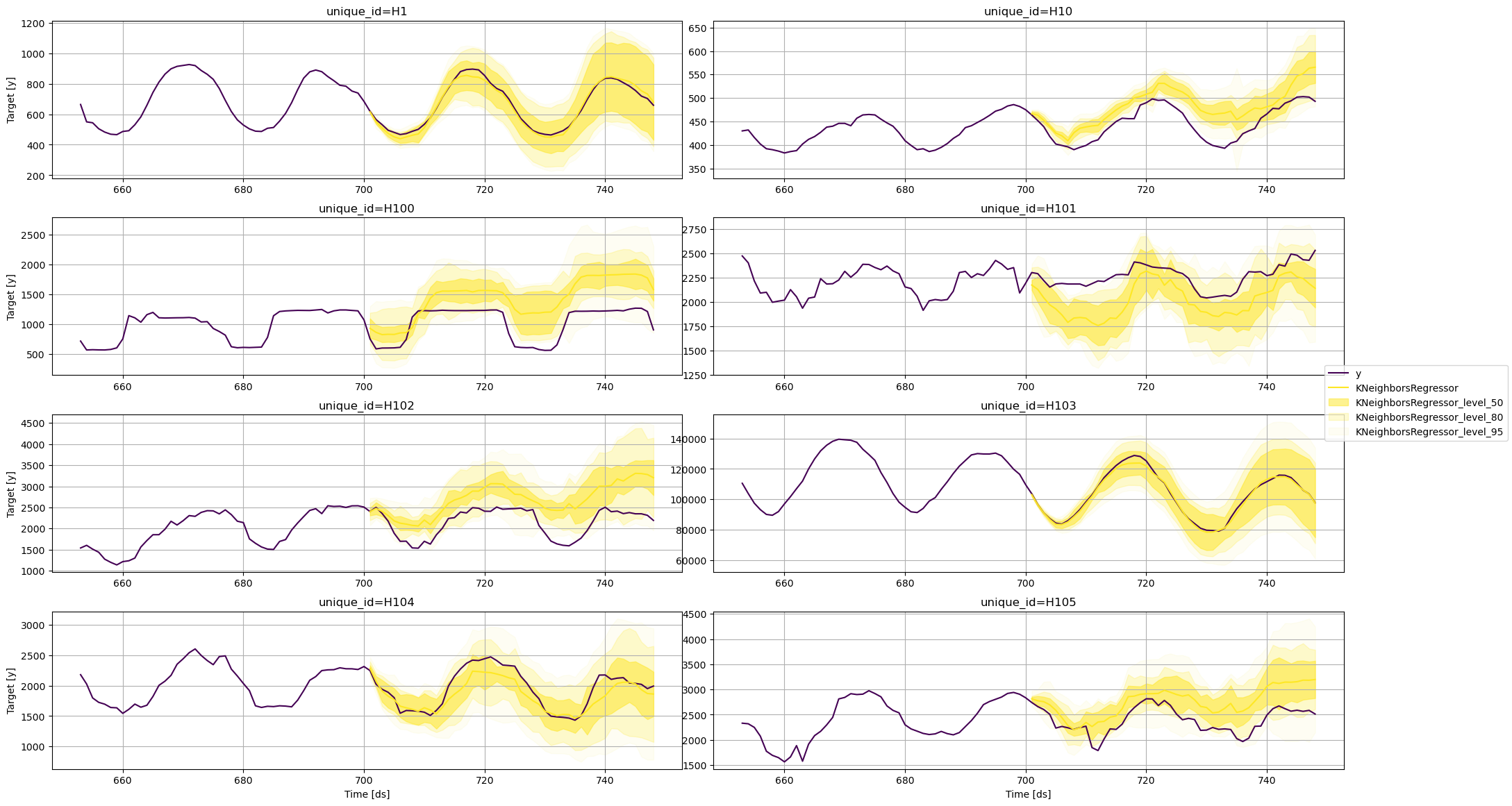
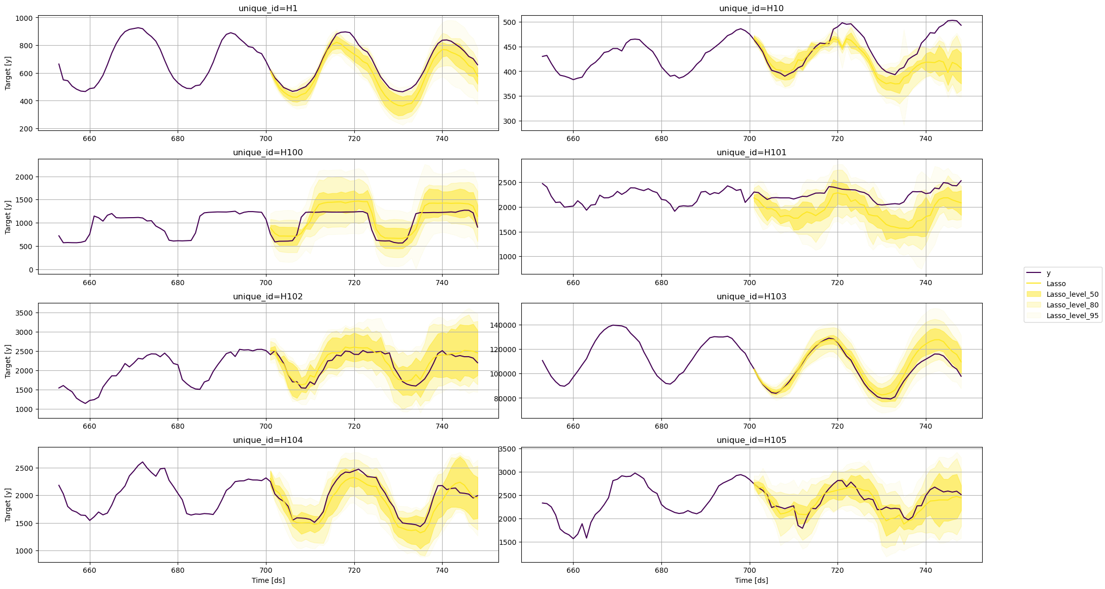
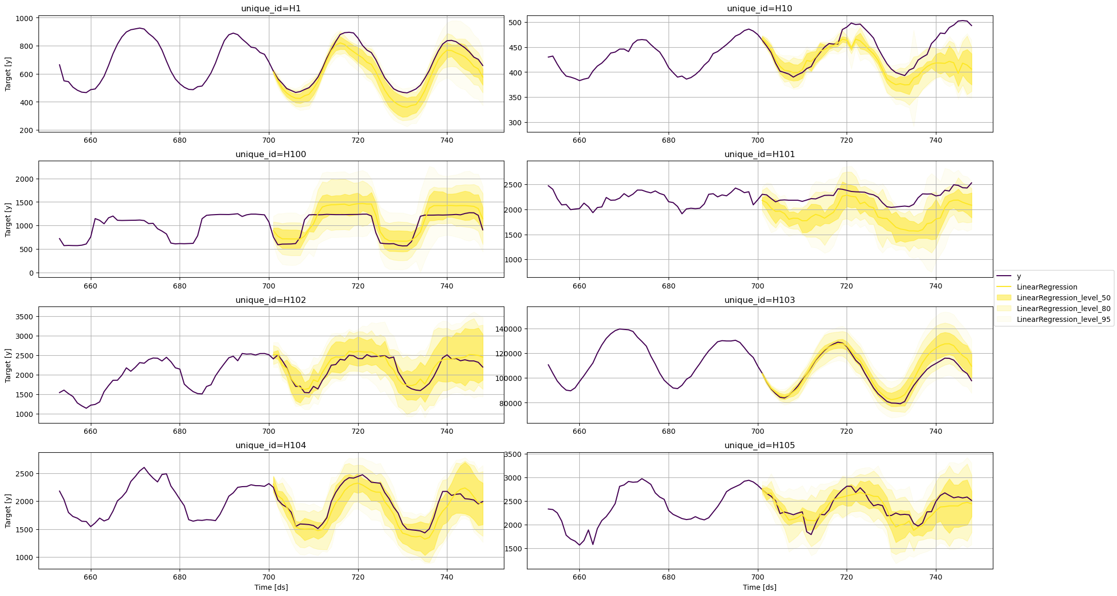
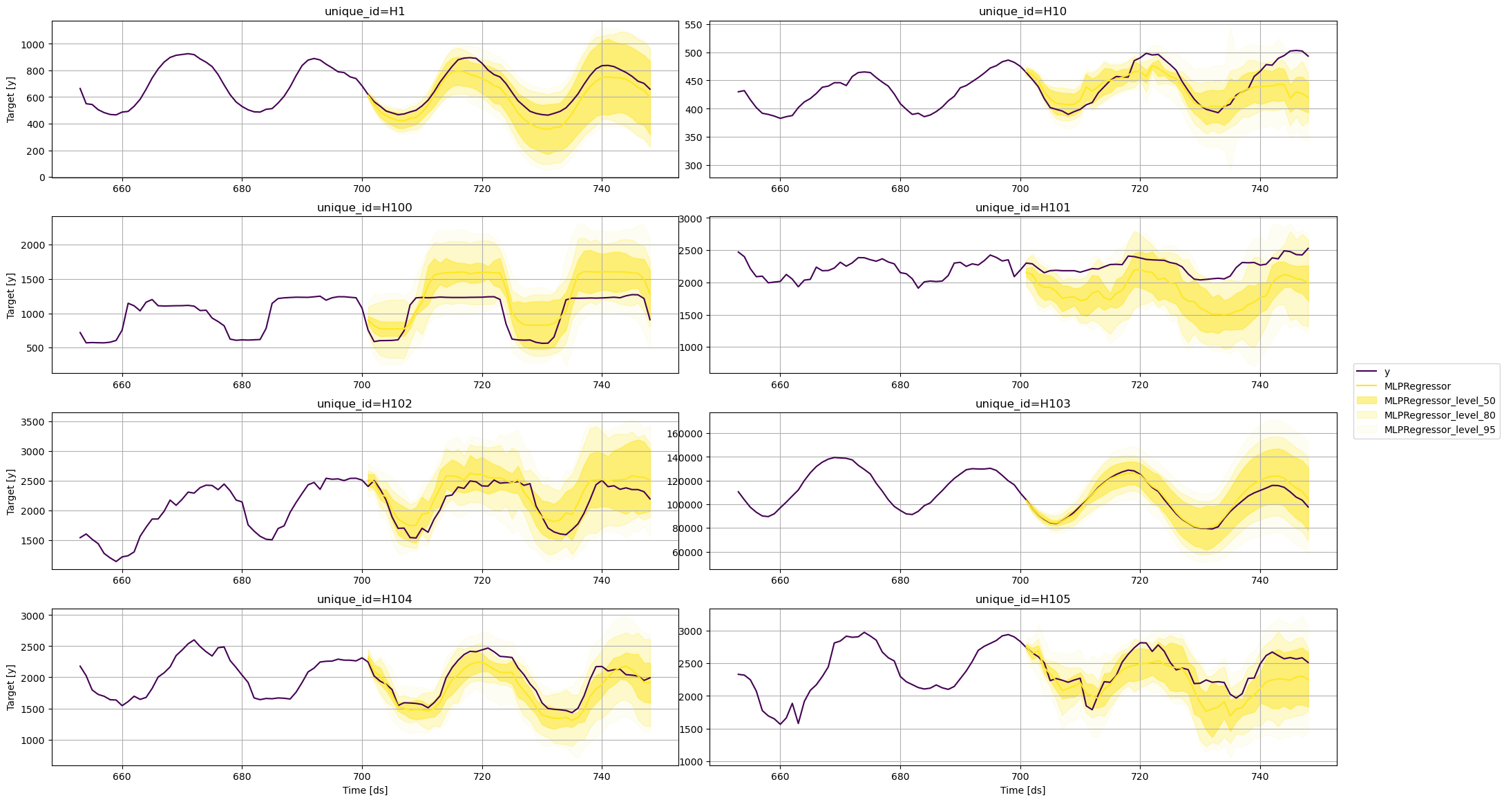
To plot the point and the prediction intervals, we’ll use the
`plot_series` function again. Notice that now we also need to specify
the model and the levels that we want to plot.
### KNeighborsRegressor
```python theme={null}
fig = plot_series(
train,
test,
plot_random=False,
models=['KNeighborsRegressor'],
level=levels,
max_insample_length=48
)
```
## Train models
MLForecast can train multiple models that follow the `sklearn` syntax
(`fit` and `predict`) on different time series efficiently.
For this example, we’ll use the following `sklearn` baseline models:
* [Lasso](https://scikit-learn.org/stable/modules/generated/sklearn.linear_model.Lasso.html)
* [LinearRegression](https://scikit-learn.org/stable/modules/generated/sklearn.linear_model.LinearRegression.html)
* [Ridge](https://scikit-learn.org/stable/modules/generated/sklearn.linear_model.Ridge.html)
* [K-Nearest
Neighbors](https://scikit-learn.org/stable/modules/generated/sklearn.neighbors.KNeighborsRegressor.html)
* [Multilayer Perceptron
(NeuralNetwork)](https://scikit-learn.org/stable/modules/generated/sklearn.neural_network.MLPRegressor.html)
To use these models, we first need to import them from `sklearn` and
then we need to instantiate them.
```python theme={null}
from mlforecast import MLForecast
from mlforecast.target_transforms import Differences
from mlforecast.utils import PredictionIntervals
from sklearn.linear_model import Lasso, LinearRegression, Ridge
from sklearn.neighbors import KNeighborsRegressor
from sklearn.neural_network import MLPRegressor
```
```python theme={null}
# Create a list of models and instantiation parameters
models = [
KNeighborsRegressor(),
Lasso(),
LinearRegression(),
MLPRegressor(),
Ridge(),
]
```
To instantiate a new MLForecast object, we need the following
parameters:
* `models`: The list of models defined in the previous step.
* `target_transforms`: Transformations to apply to the target before
computing the features. These are restored at the forecasting step.
* `lags`: Lags of the target to use as features.
```python theme={null}
mlf = MLForecast(
models=[Ridge(), Lasso(), LinearRegression(), KNeighborsRegressor(), MLPRegressor(random_state=0)],
freq=1,
target_transforms=[Differences([1])],
lags=[24 * (i+1) for i in range(7)],
)
```
Now we’re ready to generate the point forecasts and the prediction
intervals. To do this, we’ll use the `fit` method, which takes the
following arguments:
* `data`: Series data in long format.
* `id_col`: Column that identifies each series. In our case,
`unique_id`.
* `time_col`: Column that identifies each timestep, its values can be
timestamps or integers. In our case, `ds`.
* `target_col`: Column that contains the target. In our case, `y`.
* `prediction_intervals`: A `PredicitonIntervals` class. The class
takes two parameters: `n_windows` and `h`. `n_windows` represents
the number of cross-validation windows used to calibrate the
intervals and `h` is the forecast horizon. The strategy will adjust
the intervals for each horizon step, resulting in different widths
for each step.
```python theme={null}
mlf.fit(
train,
prediction_intervals=PredictionIntervals(n_windows=10, h=48),
);
```
After fitting the models, we will call the `predict` method to generate
forecasts with prediction intervals. The method takes the following
arguments:
* `horizon`: An integer that represent the forecasting horizon. In
this case, we’ll forecast the next 48 hours.
* `level`: A list of floats with the confidence levels of the
prediction intervals. For example, `level=[95]` means that the range
of values should include the actual future value with probability
95%.
```python theme={null}
levels = [50, 80, 95]
forecasts = mlf.predict(48, level=levels)
forecasts.head()
```
| | unique\_id | ds | Ridge | Lasso | LinearRegression | KNeighborsRegressor | MLPRegressor | Ridge-lo-95 | Ridge-lo-80 | Ridge-lo-50 | ... | KNeighborsRegressor-lo-50 | KNeighborsRegressor-hi-50 | KNeighborsRegressor-hi-80 | KNeighborsRegressor-hi-95 | MLPRegressor-lo-95 | MLPRegressor-lo-80 | MLPRegressor-lo-50 | MLPRegressor-hi-50 | MLPRegressor-hi-80 | MLPRegressor-hi-95 |
| - | ---------- | --- | ---------- | ---------- | ---------------- | ------------------- | ------------ | ----------- | ----------- | ----------- | --- | ------------------------- | ------------------------- | ------------------------- | ------------------------- | ------------------ | ------------------ | ------------------ | ------------------ | ------------------ | ------------------ |
| 0 | H1 | 701 | 612.418170 | 612.418079 | 612.418170 | 615.2 | 612.651532 | 590.473256 | 594.326570 | 603.409944 | ... | 609.45 | 620.95 | 627.20 | 631.310 | 584.736193 | 591.084898 | 597.462107 | 627.840957 | 634.218166 | 640.566870 |
| 1 | H1 | 702 | 552.309298 | 552.308073 | 552.309298 | 551.6 | 548.791801 | 498.721501 | 518.433843 | 532.710850 | ... | 535.85 | 567.35 | 569.16 | 597.525 | 497.308756 | 500.417799 | 515.452396 | 582.131207 | 597.165804 | 600.274847 |
| 2 | H1 | 703 | 494.943384 | 494.943367 | 494.943384 | 509.6 | 490.226796 | 448.253304 | 463.266064 | 475.006125 | ... | 492.70 | 526.50 | 530.92 | 544.180 | 424.587658 | 436.042788 | 448.682502 | 531.771091 | 544.410804 | 555.865935 |
| 3 | H1 | 704 | 462.815779 | 462.815363 | 462.815779 | 474.6 | 459.619069 | 409.975219 | 422.243593 | 436.128272 | ... | 451.80 | 497.40 | 510.26 | 525.500 | 379.291083 | 392.580306 | 413.353178 | 505.884959 | 526.657832 | 539.947054 |
| 4 | H1 | 705 | 440.141034 | 440.140586 | 440.141034 | 451.6 | 438.091712 | 377.999588 | 392.523016 | 413.474795 | ... | 427.40 | 475.80 | 488.96 | 503.945 | 348.618034 | 362.503767 | 386.303325 | 489.880099 | 513.679657 | 527.565389 |
```python theme={null}
test = test.merge(forecasts, how='left', on=['unique_id', 'ds'])
```
## Plot prediction intervals
To plot the point and the prediction intervals, we’ll use the
`plot_series` function again. Notice that now we also need to specify
the model and the levels that we want to plot.
### KNeighborsRegressor
```python theme={null}
fig = plot_series(
train,
test,
plot_random=False,
models=['KNeighborsRegressor'],
level=levels,
max_insample_length=48
)
```
 ### Lasso
```python theme={null}
fig = plot_series(
train,
test,
plot_random=False,
models=['Lasso'],
level=levels,
max_insample_length=48
)
```
### Lasso
```python theme={null}
fig = plot_series(
train,
test,
plot_random=False,
models=['Lasso'],
level=levels,
max_insample_length=48
)
```
 ### Linear Regression
```python theme={null}
fig = plot_series(
train,
test,
plot_random=False,
models=['LinearRegression'],
level=levels,
max_insample_length=48
)
```
### Linear Regression
```python theme={null}
fig = plot_series(
train,
test,
plot_random=False,
models=['LinearRegression'],
level=levels,
max_insample_length=48
)
```
 ### MLPRegressor
```python theme={null}
fig = plot_series(
train,
test,
plot_random=False,
models=['MLPRegressor'],
level=levels,
max_insample_length=48
)
```
### MLPRegressor
```python theme={null}
fig = plot_series(
train,
test,
plot_random=False,
models=['MLPRegressor'],
level=levels,
max_insample_length=48
)
```
 ### Ridge
```python theme={null}
fig = plot_series(
train,
test,
plot_random=False,
models=['Ridge'],
level=levels,
max_insample_length=48
)
```
### Ridge
```python theme={null}
fig = plot_series(
train,
test,
plot_random=False,
models=['Ridge'],
level=levels,
max_insample_length=48
)
```
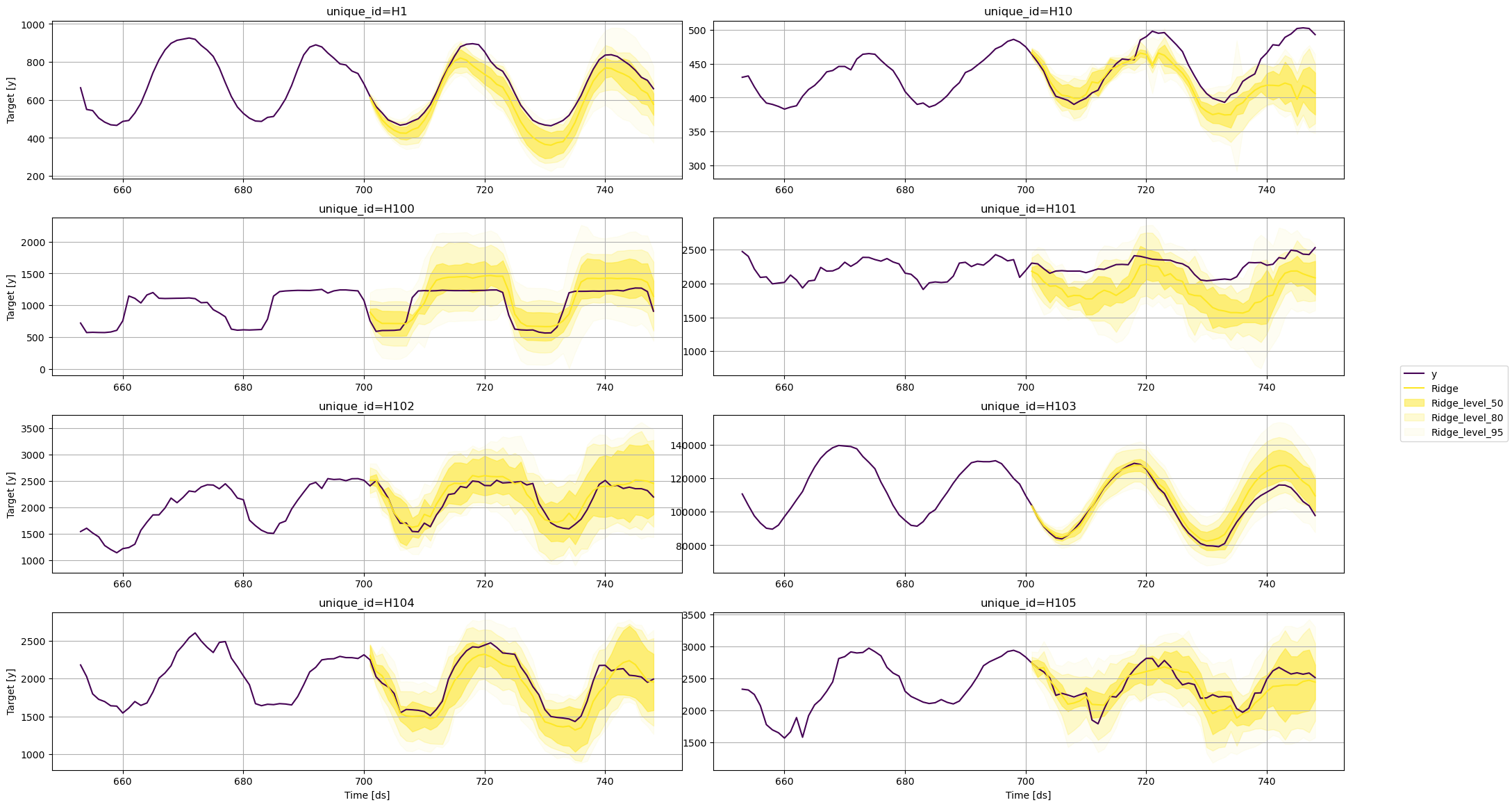 From these plots, we can conclude that the uncertainty around each
forecast varies according to the model that is being used. For the same
time series, one model can predict a wider range of possible future
values than others.
## References
* [Kamile Stankeviciute, Ahmed M. Alaa and Mihaela van der Schaar
(2021). “Conformal Time-Series
Forecasting”](https://proceedings.neurips.cc/paper/2021/file/312f1ba2a72318edaaa995a67835fad5-Paper.pdf)
* [Rob J. Hyndman and George Athanasopoulos (2018). “Forecasting
principles and practice, The Statistical Forecasting
Perspective”](https://otexts.com/fpp3/perspective.html).
From these plots, we can conclude that the uncertainty around each
forecast varies according to the model that is being used. For the same
time series, one model can predict a wider range of possible future
values than others.
## References
* [Kamile Stankeviciute, Ahmed M. Alaa and Mihaela van der Schaar
(2021). “Conformal Time-Series
Forecasting”](https://proceedings.neurips.cc/paper/2021/file/312f1ba2a72318edaaa995a67835fad5-Paper.pdf)
* [Rob J. Hyndman and George Athanasopoulos (2018). “Forecasting
principles and practice, The Statistical Forecasting
Perspective”](https://otexts.com/fpp3/perspective.html).