> ## Documentation Index
> Fetch the complete documentation index at: https://nixtlaverse.nixtla.io/llms.txt
> Use this file to discover all available pages before exploring further.
# Cross validation | MLForecast
> In this example, we’ll implement time series cross-validation to
> evaluate model’s performance.
> **Prerequesites**
>
> This tutorial assumes basic familiarity with `MLForecast`. For a
> minimal example visit the [Quick
> Start](https://nixtlaverse.nixtla.io/mlforecast/docs/getting-started/quick_start_local.html)
## Introduction
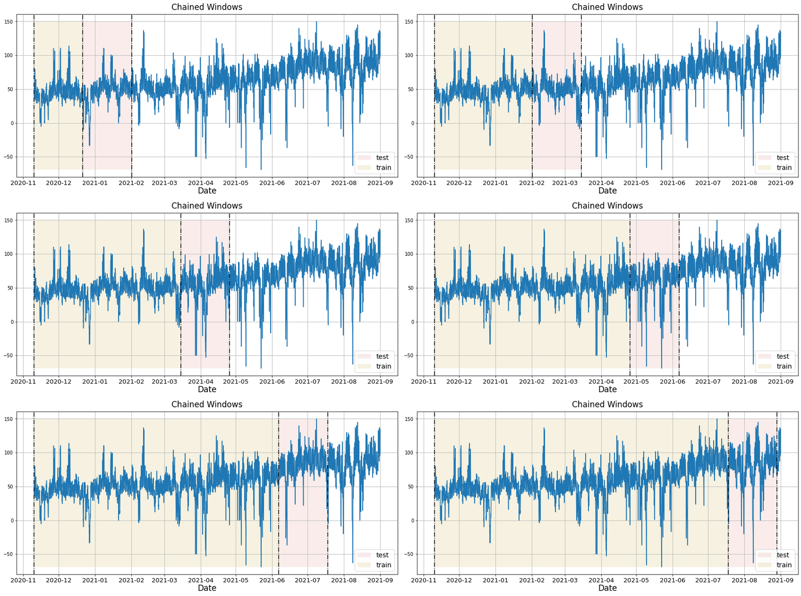
Time series cross-validation is a method for evaluating how a model
would have performed in the past. It works by defining a sliding window
across the historical data and predicting the period following it.
[MLForecast](https://nixtlaverse.nixtla.io/mlforecast/) has an
implementation of time series cross-validation that is fast and easy to
use. This implementation makes cross-validation an efficient operation,
which makes it less time-consuming. In this notebook, we’ll use it on a
subset of the [M4
Competition](https://www.sciencedirect.com/science/article/pii/S0169207019301128)
hourly dataset.
**Outline:**
1. Install libraries
2. Load and explore data
3. Train model
4. Perform time series cross-validation
5. Evaluate results
> **Tip**
>
> You can use Colab to run this Notebook interactively
>
>
>  >
## Install libraries
We assume that you have `MLForecast` already installed. If not, check
this guide for instructions on [how to install
MLForecast](https://nixtlaverse.nixtla.io/mlforecast/docs/getting-started/install.html)
Install the necessary packages with `pip install mlforecast`.
```python theme={null}
import pandas as pd
from utilsforecast.plotting import plot_series
from mlforecast import MLForecast # required to instantiate MLForecast object and use cross-validation method
```
## Load and explore the data
As stated in the introduction, we’ll use the M4 Competition hourly
dataset. We’ll first import the data from an URL using `pandas`.
```python theme={null}
Y_df = pd.read_csv('https://datasets-nixtla.s3.amazonaws.com/m4-hourly.csv') # load the data
Y_df.head()
```
| | unique\_id | ds | y |
| - | ---------- | -- | ----- |
| 0 | H1 | 1 | 605.0 |
| 1 | H1 | 2 | 586.0 |
| 2 | H1 | 3 | 586.0 |
| 3 | H1 | 4 | 559.0 |
| 4 | H1 | 5 | 511.0 |
The input to `MLForecast` is a data frame in [long
format](https://www.theanalysisfactor.com/wide-and-long-data/) with
three columns: `unique_id`, `ds` and `y`:
* The `unique_id` (string, int, or category) represents an identifier
for the series.
* The `ds` (datestamp or int) column should be either an integer
indexing time or a datestamp in format YYYY-MM-DD or YYYY-MM-DD
HH:MM:SS.
* The `y` (numeric) represents the measurement we wish to forecast.
The data in this example already has this format, so no changes are
needed.
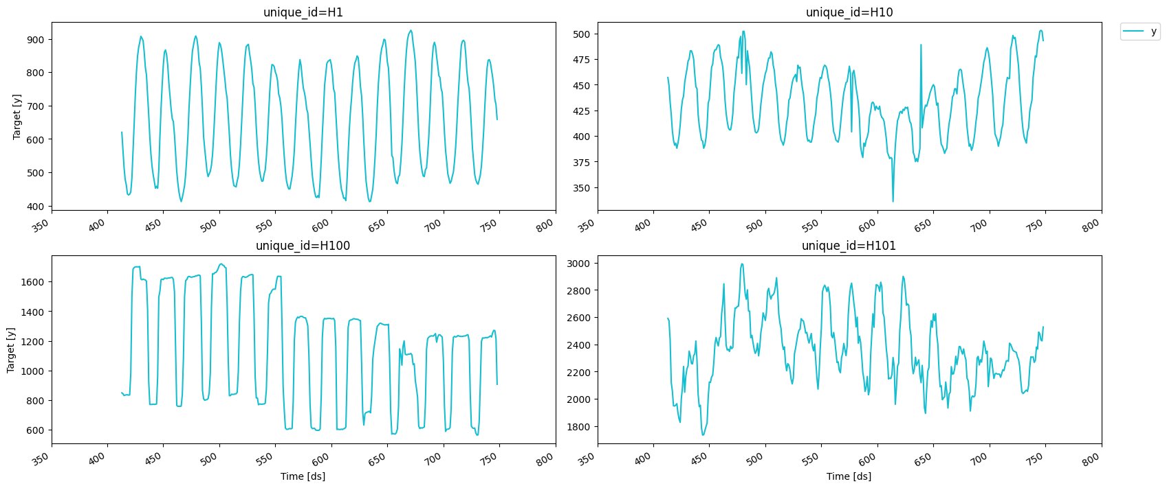
We can plot the time series we’ll work with using the following
function.
```python theme={null}
fig = plot_series(Y_df, max_ids=4, plot_random=False, max_insample_length=24 * 14)
```
>
## Install libraries
We assume that you have `MLForecast` already installed. If not, check
this guide for instructions on [how to install
MLForecast](https://nixtlaverse.nixtla.io/mlforecast/docs/getting-started/install.html)
Install the necessary packages with `pip install mlforecast`.
```python theme={null}
import pandas as pd
from utilsforecast.plotting import plot_series
from mlforecast import MLForecast # required to instantiate MLForecast object and use cross-validation method
```
## Load and explore the data
As stated in the introduction, we’ll use the M4 Competition hourly
dataset. We’ll first import the data from an URL using `pandas`.
```python theme={null}
Y_df = pd.read_csv('https://datasets-nixtla.s3.amazonaws.com/m4-hourly.csv') # load the data
Y_df.head()
```
| | unique\_id | ds | y |
| - | ---------- | -- | ----- |
| 0 | H1 | 1 | 605.0 |
| 1 | H1 | 2 | 586.0 |
| 2 | H1 | 3 | 586.0 |
| 3 | H1 | 4 | 559.0 |
| 4 | H1 | 5 | 511.0 |
The input to `MLForecast` is a data frame in [long
format](https://www.theanalysisfactor.com/wide-and-long-data/) with
three columns: `unique_id`, `ds` and `y`:
* The `unique_id` (string, int, or category) represents an identifier
for the series.
* The `ds` (datestamp or int) column should be either an integer
indexing time or a datestamp in format YYYY-MM-DD or YYYY-MM-DD
HH:MM:SS.
* The `y` (numeric) represents the measurement we wish to forecast.
The data in this example already has this format, so no changes are
needed.
We can plot the time series we’ll work with using the following
function.
```python theme={null}
fig = plot_series(Y_df, max_ids=4, plot_random=False, max_insample_length=24 * 14)
```
 ## Define forecast object
For this example, we’ll use LightGBM. We first need to import it and
then we need to instantiate a new
[MLForecast](https://nixtlaverse.nixtla.io/mlforecast/forecast.html#mlforecast)
object.
In this example, we are only using `differences` and `lags` to produce
features. See [the full
documentation](https://nixtlaverse.nixtla.io/mlforecast/index.html) to
see all available features.
Any settings are passed into the constructor. Then you call its `fit`
method and pass in the historical data frame `df`.
```python theme={null}
import lightgbm as lgb
from mlforecast.target_transforms import Differences
```
```python theme={null}
models = [lgb.LGBMRegressor(verbosity=-1)]
mlf = MLForecast(
models=models,
freq=1,# our series have integer timestamps, so we'll just add 1 in every timestep,
target_transforms=[Differences([24])],
lags=range(1, 25)
)
```
## Perform time series cross-validation
Once the `MLForecast` object has been instantiated, we can use the
[cross\_validation
method](https://nixtlaverse.nixtla.io/mlforecast/forecast#method-cross-validation)
For this particular example, we’ll use 3 windows of 24 hours.
```python theme={null}
cv_df = mlf.cross_validation(
df=Y_df,
h=24,
n_windows=3,
)
```
The crossvalidation\_df object is a new data frame that includes the
following columns:
* `unique_id`: identifies each time series.
* `ds`: datestamp or temporal index.
* `cutoff`: the last datestamp or temporal index for the `n_windows`.
* `y`: true value
* `"model"`: columns with the model’s name and fitted value.
```python theme={null}
cv_df.head()
```
| | unique\_id | ds | cutoff | y | LGBMRegressor |
| - | ---------- | --- | ------ | ----- | ------------- |
| 0 | H1 | 677 | 676 | 691.0 | 673.703191 |
| 1 | H1 | 678 | 676 | 618.0 | 552.306270 |
| 2 | H1 | 679 | 676 | 563.0 | 541.778027 |
| 3 | H1 | 680 | 676 | 529.0 | 502.778027 |
| 4 | H1 | 681 | 676 | 504.0 | 480.778027 |
We’ll now plot the forecast for each cutoff period.
```python theme={null}
import matplotlib.pyplot as plt
```
```python theme={null}
def plot_cv(df, df_cv, uid, fname, last_n=24 * 14):
cutoffs = df_cv.query('unique_id == @uid')['cutoff'].unique()
fig, ax = plt.subplots(nrows=len(cutoffs), ncols=1, figsize=(14, 6), gridspec_kw=dict(hspace=0.8))
for cutoff, axi in zip(cutoffs, ax.flat):
df.query('unique_id == @uid').tail(last_n).set_index('ds').plot(ax=axi, title=uid, y='y')
df_cv.query('unique_id == @uid & cutoff == @cutoff').set_index('ds').plot(ax=axi, title=uid, y='LGBMRegressor')
fig.savefig(fname, bbox_inches='tight')
plt.close()
```
```python theme={null}
plot_cv(Y_df, cv_df, 'H1', '../../figs/cross_validation__predictions.png')
```
## Define forecast object
For this example, we’ll use LightGBM. We first need to import it and
then we need to instantiate a new
[MLForecast](https://nixtlaverse.nixtla.io/mlforecast/forecast.html#mlforecast)
object.
In this example, we are only using `differences` and `lags` to produce
features. See [the full
documentation](https://nixtlaverse.nixtla.io/mlforecast/index.html) to
see all available features.
Any settings are passed into the constructor. Then you call its `fit`
method and pass in the historical data frame `df`.
```python theme={null}
import lightgbm as lgb
from mlforecast.target_transforms import Differences
```
```python theme={null}
models = [lgb.LGBMRegressor(verbosity=-1)]
mlf = MLForecast(
models=models,
freq=1,# our series have integer timestamps, so we'll just add 1 in every timestep,
target_transforms=[Differences([24])],
lags=range(1, 25)
)
```
## Perform time series cross-validation
Once the `MLForecast` object has been instantiated, we can use the
[cross\_validation
method](https://nixtlaverse.nixtla.io/mlforecast/forecast#method-cross-validation)
For this particular example, we’ll use 3 windows of 24 hours.
```python theme={null}
cv_df = mlf.cross_validation(
df=Y_df,
h=24,
n_windows=3,
)
```
The crossvalidation\_df object is a new data frame that includes the
following columns:
* `unique_id`: identifies each time series.
* `ds`: datestamp or temporal index.
* `cutoff`: the last datestamp or temporal index for the `n_windows`.
* `y`: true value
* `"model"`: columns with the model’s name and fitted value.
```python theme={null}
cv_df.head()
```
| | unique\_id | ds | cutoff | y | LGBMRegressor |
| - | ---------- | --- | ------ | ----- | ------------- |
| 0 | H1 | 677 | 676 | 691.0 | 673.703191 |
| 1 | H1 | 678 | 676 | 618.0 | 552.306270 |
| 2 | H1 | 679 | 676 | 563.0 | 541.778027 |
| 3 | H1 | 680 | 676 | 529.0 | 502.778027 |
| 4 | H1 | 681 | 676 | 504.0 | 480.778027 |
We’ll now plot the forecast for each cutoff period.
```python theme={null}
import matplotlib.pyplot as plt
```
```python theme={null}
def plot_cv(df, df_cv, uid, fname, last_n=24 * 14):
cutoffs = df_cv.query('unique_id == @uid')['cutoff'].unique()
fig, ax = plt.subplots(nrows=len(cutoffs), ncols=1, figsize=(14, 6), gridspec_kw=dict(hspace=0.8))
for cutoff, axi in zip(cutoffs, ax.flat):
df.query('unique_id == @uid').tail(last_n).set_index('ds').plot(ax=axi, title=uid, y='y')
df_cv.query('unique_id == @uid & cutoff == @cutoff').set_index('ds').plot(ax=axi, title=uid, y='LGBMRegressor')
fig.savefig(fname, bbox_inches='tight')
plt.close()
```
```python theme={null}
plot_cv(Y_df, cv_df, 'H1', '../../figs/cross_validation__predictions.png')
```
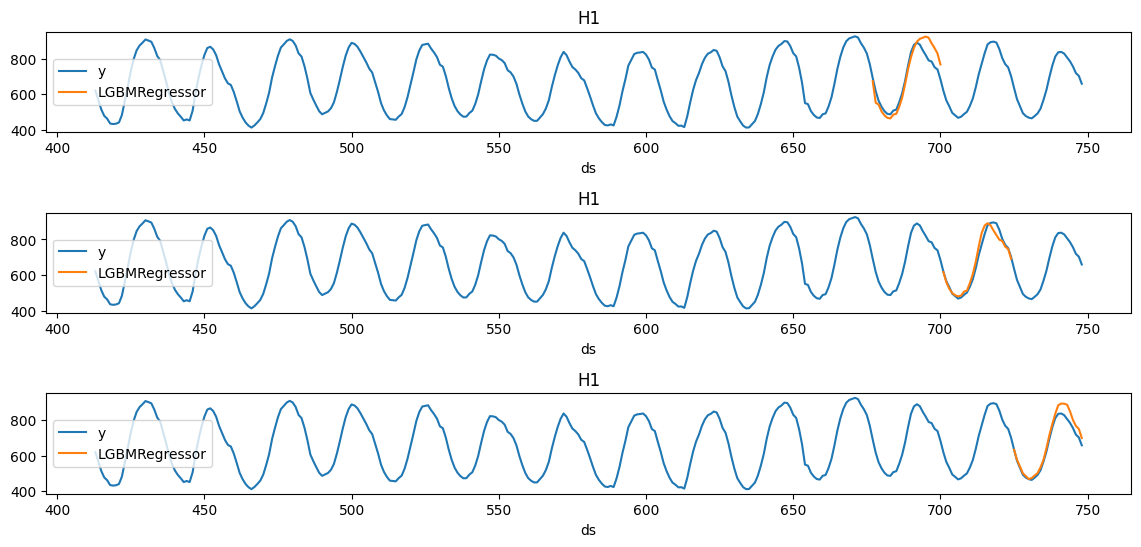 Notice that in each cutoff period, we generated a forecast for the next
24 hours using only the data `y` before said period.
## Evaluate results
We can now compute the accuracy of the forecast using an appropiate
accuracy metric. Here we’ll use the [Root Mean Squared Error
(RMSE).](https://en.wikipedia.org/wiki/Root-mean-square_deviation) To do
this, we can use `utilsforecast`, a Python library developed by Nixtla
that includes a function to compute the RMSE.
```python theme={null}
from utilsforecast.evaluation import evaluate
from utilsforecast.losses import rmse
```
```python theme={null}
cv_rmse = evaluate(
cv_df.drop(columns='cutoff'),
metrics=[rmse],
agg_fn='mean',
)
print(f"RMSE using cross-validation: {cv_rmse['LGBMRegressor'].item():.1f}")
```
```text theme={null}
RMSE using cross-validation: 269.0
```
This measure should better reflect the predictive abilities of our
model, since it used different time periods to test its accuracy.
## References
[Rob J. Hyndman and George Athanasopoulos (2018). “Forecasting
principles and practice, Time series
cross-validation”](https://otexts.com/fpp3/tscv.html).
Notice that in each cutoff period, we generated a forecast for the next
24 hours using only the data `y` before said period.
## Evaluate results
We can now compute the accuracy of the forecast using an appropiate
accuracy metric. Here we’ll use the [Root Mean Squared Error
(RMSE).](https://en.wikipedia.org/wiki/Root-mean-square_deviation) To do
this, we can use `utilsforecast`, a Python library developed by Nixtla
that includes a function to compute the RMSE.
```python theme={null}
from utilsforecast.evaluation import evaluate
from utilsforecast.losses import rmse
```
```python theme={null}
cv_rmse = evaluate(
cv_df.drop(columns='cutoff'),
metrics=[rmse],
agg_fn='mean',
)
print(f"RMSE using cross-validation: {cv_rmse['LGBMRegressor'].item():.1f}")
```
```text theme={null}
RMSE using cross-validation: 269.0
```
This measure should better reflect the predictive abilities of our
model, since it used different time periods to test its accuracy.
## References
[Rob J. Hyndman and George Athanasopoulos (2018). “Forecasting
principles and practice, Time series
cross-validation”](https://otexts.com/fpp3/tscv.html).