[ndarray](#numpy.ndarray) | Array with the time series. | *required* |
| `season_length` | [int](#int) | Length of the seasonal pattern. | *required* |
| `max_d` | [int](#int) | Maximum number of differences to consider. Defaults to 1. | 1 |
**Returns:**
| Name | Type | Description |
| ----- | ------------------------ | --------------------------------------- |
| `int` | [int](#int) | Optimal number of seasonal differences. |
### `num_diffs`
```python theme={null}
num_diffs(x, max_d=1)
```
Determine the optimal number of non-seasonal differences for stationarity.
Uses the KPSS (Kwiatkowski-Phillips-Schmidt-Shin) test to determine how many
times the series needs to be differenced to achieve stationarity. The function
applies differencing iteratively until the KPSS statistic falls below the
threshold or the maximum number of differences is reached.
**Parameters:**
| Name | Type | Description | Default |
| ------- | -------------------------------------- | --------------------------------------------------------- | -------------- |
| `x` | [ndarray](#numpy.ndarray) | Array with the time series. | *required* |
| `max_d` | [int](#int) | Maximum number of differences to consider. Defaults to 1. | 1 |
**Returns:**
| Name | Type | Description |
| ----- | ------------------------ | ------------------------------ |
| `int` | [int](#int) | Optimal number of differences. |
### `diff`
```python theme={null}
diff(x, d)
```
Subtract previous values of the series
**Parameters:**
| Name | Type | Description | Default |
| ---- | -------------------------------------- | --------------------------- | ---------- |
| `x` | [ndarray](#numpy.ndarray) | Array with the time series. | *required* |
| `d` | [int](#int) | Lag to subtract | *required* |
**Returns:**
| Type | Description |
| -------------------------------------- | ------------------------------------ |
| [ndarray](#numpy.ndarray) | np.ndarray: Differenced time series. |
# Expanding
Source: https://nixtlaverse.nixtla.io/coreforecast/expanding
Compute expanding mean, std, min, max, and quantile
##
### `expanding_mean`
```python theme={null}
expanding_mean(x, skipna=False)
```
Compute the expanding\_mean of the input array.
**Parameters:**
| Name | Type | Description | Default |
| -------- | ----------------------- | -------------------------------------------------------------------------------------------------------------------------------------------------------------------------------------------------------------------------- | ---------- |
| `x` | np.ndarray | Input array. | *required* |
| `skipna` | bool | If True, exclude NaN values from calculations. When False (default), any NaN value causes the result to be NaN, maintaining backwards compatibility. When True, NaN values are ignored (matching pandas default behavior). | *required* |
**Returns:**
| Type | Description |
| ---------------------------------------------- | ----------- |
| np.ndarray: Array with the expanding statistic | |
**Examples:**
```pycon theme={null}
>>> import numpy as np
>>> x = np.array([1.0, 2.0, np.nan, 4.0, 5.0])
>>> # Default behavior: NaN propagates
>>> expanding_mean(x)
array([1., 1.5, nan, nan, nan])
>>> # With skipna=True: NaN values are excluded
>>> expanding_mean(x, skipna=True)
array([1., 1.5, 1.5, 2.33..., 3.0])
```
### `expanding_std`
```python theme={null}
expanding_std(x, skipna=False)
```
Compute the expanding\_std of the input array.
**Parameters:**
| Name | Type | Description | Default |
| -------- | ----------------------- | -------------------------------------------------------------------------------------------------------------------------------------------------------------------------------------------------------------------------- | ---------- |
| `x` | np.ndarray | Input array. | *required* |
| `skipna` | bool | If True, exclude NaN values from calculations. When False (default), any NaN value causes the result to be NaN, maintaining backwards compatibility. When True, NaN values are ignored (matching pandas default behavior). | *required* |
**Returns:**
| Type | Description |
| ---------------------------------------------- | ----------- |
| np.ndarray: Array with the expanding statistic | |
**Examples:**
```pycon theme={null}
>>> import numpy as np
>>> x = np.array([1.0, 2.0, np.nan, 4.0, 5.0])
>>> # Default behavior: NaN propagates
>>> expanding_std(x)
array([1., 1.5, nan, nan, nan])
>>> # With skipna=True: NaN values are excluded
>>> expanding_std(x, skipna=True)
array([1., 1.5, 1.5, 2.33..., 3.0])
```
### `expanding_min`
```python theme={null}
expanding_min(x, skipna=False)
```
Compute the expanding\_min of the input array.
**Parameters:**
| Name | Type | Description | Default |
| -------- | ----------------------- | -------------------------------------------------------------------------------------------------------------------------------------------------------------------------------------------------------------------------- | ---------- |
| `x` | np.ndarray | Input array. | *required* |
| `skipna` | bool | If True, exclude NaN values from calculations. When False (default), any NaN value causes the result to be NaN, maintaining backwards compatibility. When True, NaN values are ignored (matching pandas default behavior). | *required* |
**Returns:**
| Type | Description |
| ---------------------------------------------- | ----------- |
| np.ndarray: Array with the expanding statistic | |
**Examples:**
```pycon theme={null}
>>> import numpy as np
>>> x = np.array([1.0, 2.0, np.nan, 4.0, 5.0])
>>> # Default behavior: NaN propagates
>>> expanding_min(x)
array([1., 1.5, nan, nan, nan])
>>> # With skipna=True: NaN values are excluded
>>> expanding_min(x, skipna=True)
array([1., 1.5, 1.5, 2.33..., 3.0])
```
### `expanding_max`
```python theme={null}
expanding_max(x, skipna=False)
```
Compute the expanding\_max of the input array.
**Parameters:**
| Name | Type | Description | Default |
| -------- | ----------------------- | -------------------------------------------------------------------------------------------------------------------------------------------------------------------------------------------------------------------------- | ---------- |
| `x` | np.ndarray | Input array. | *required* |
| `skipna` | bool | If True, exclude NaN values from calculations. When False (default), any NaN value causes the result to be NaN, maintaining backwards compatibility. When True, NaN values are ignored (matching pandas default behavior). | *required* |
**Returns:**
| Type | Description |
| ---------------------------------------------- | ----------- |
| np.ndarray: Array with the expanding statistic | |
**Examples:**
```pycon theme={null}
>>> import numpy as np
>>> x = np.array([1.0, 2.0, np.nan, 4.0, 5.0])
>>> # Default behavior: NaN propagates
>>> expanding_max(x)
array([1., 1.5, nan, nan, nan])
>>> # With skipna=True: NaN values are excluded
>>> expanding_max(x, skipna=True)
array([1., 1.5, 1.5, 2.33..., 3.0])
```
### `expanding_quantile`
```python theme={null}
expanding_quantile(x, p, skipna=False)
```
Compute the expanding\_quantile of the input array.
**Parameters:**
| Name | Type | Description | Default |
| -------- | -------------------------------------- | -------------------------------------------------------------------------------------------------------------------------------------------------------------------------------------------------------------------------- | ------------------ |
| `x` | [ndarray](#numpy.ndarray) | Input array. | *required* |
| `p` | [float](#float) | Quantile to compute. | *required* |
| `skipna` | [bool](#bool) | If True, exclude NaN values from calculations. When False (default), any NaN value causes the result to be NaN, maintaining backwards compatibility. When True, NaN values are ignored (matching pandas default behavior). | False |
**Returns:**
| Type | Description |
| -------------------------------------- | ---------------------------------------------- |
| [ndarray](#numpy.ndarray) | np.ndarray: Array with the expanding statistic |
**Examples:**
```pycon theme={null}
>>> import numpy as np
>>> x = np.array([1.0, 2.0, np.nan, 4.0, 5.0])
>>> # Default behavior: NaN propagates
>>> expanding_quantile(x, 0.5)
array([1., 1.5, nan, nan, nan])
>>> # With skipna=True: NaN values are excluded
>>> expanding_quantile(x, 0.5, skipna=True)
array([1., 1.5, 1.5, 2., 2.5])
```
# Exponentially weighted
Source: https://nixtlaverse.nixtla.io/coreforecast/exponentially_weighted
Compute exponentially weighted mean
##
### `exponentially_weighted_mean`
```python theme={null}
exponentially_weighted_mean(x, alpha, skipna=False)
```
Compute the exponentially weighted mean of the input array.
**Parameters:**
| Name | Type | Description | Default |
| -------- | -------------------------------------- | ----------------------------------------------------------------------------------------------------------------------------------------------------------------------------------------------------------------------------------------------------------------------------------------- | ------------------ |
| `x` | [ndarray](#numpy.ndarray) | Input array. | *required* |
| `alpha` | [float](#float) | Weight parameter. | *required* |
| `skipna` | [bool](#bool) | If True, exclude NaN values from calculations using forward-fill behavior. When False (default), any NaN value causes the result to be NaN, maintaining backwards compatibility. When True, the last valid value is forward-filled through NaN values (matching pandas default behavior). | False |
**Returns:**
| Type | Description |
| -------------------------------------- | ------------------------------------------------------- |
| [ndarray](#numpy.ndarray) | np.ndarray: Array with the exponentially weighted mean. |
**Examples:**
```pycon theme={null}
>>> import numpy as np
>>> x = np.array([1.0, 2.0, np.nan, 4.0, 5.0])
>>> # Default behavior: NaN propagates
>>> exponentially_weighted_mean(x, alpha=0.5)
array([1., 1.5, nan, nan, nan])
>>> # With skipna=True: forward-fill through NaN
>>> exponentially_weighted_mean(x, alpha=0.5, skipna=True)
array([1., 1.5, 1.5, 2.75, 3.875])
```
# Grouped Array
Source: https://nixtlaverse.nixtla.io/coreforecast/grouped_array
Group arrays by a categorical variable
# coreforecast
Source: https://nixtlaverse.nixtla.io/coreforecast/index
Fast implementations of common forecasting routines
## Motivation
At Nixtla we have implemented several libraries to deal with time series data. We often have to apply some transformation over all of the series, which can prove time consuming even for simple operations like performing some kind of scaling.
We've used [numba](https://numba.pydata.org/) to speed up our expensive computations, however that comes with other issues such as cold starts and more dependencies (LLVM). That's why we developed this library, which implements several operators in C++ to transform time series data (or other kind of data that can be thought of as independent groups), with the possibility to use multithreading to get the best performance possible.
You probably won't need to use this library directly but rather use one of our higher level libraries like [mlforecast](https://nixtlaverse.nixtla.io/mlforecast/docs/how-to-guides/lag_transforms_guide.html#built-in-transformations-experimental), which will use this library under the hood. If you're interested on using this library directly (only depends on numpy) you should continue reading.
## Installation
### PyPI
```python theme={null}
pip install coreforecast
```
### conda-forge
```python theme={null}
conda install -c conda-forge coreforecast
```
## Minimal example
The base data structure is the "grouped array" which holds two numpy 1d arrays:
* **data**: values of the series.
* **indptr**: series boundaries such that `data[indptr[i] : indptr[i + 1]]` returns the `i-th` series. For example, if you have two series of sizes 5 and 10 the indptr would be \[0, 5, 15].
```python theme={null}
import numpy as np
from coreforecast.grouped_array import GroupedArray
data = np.arange(10)
indptr = np.array([0, 3, 10])
ga = GroupedArray(data, indptr)
```
Once you have this structure you can run any of the provided transformations, for example:
```python theme={null}
from coreforecast.lag_transforms import ExpandingMean
from coreforecast.scalers import LocalStandardScaler
exp_mean = ExpandingMean(lag=1).transform(ga)
scaler = LocalStandardScaler().fit(ga)
standardized = scaler.transform(ga)
```
## Single-array functions
We've also implemented some functions that work on single arrays, you can refer to the following pages:
* [differences](https://nixtlaverse.nixtla.io/coreforecast/differences)
* [scalers](https://nixtlaverse.nixtla.io/coreforecast/scalers)
* [seasonal](https://nixtlaverse.nixtla.io/coreforecast/seasonal)
* [rolling](https://nixtlaverse.nixtla.io/coreforecast/rolling)
* [expanding](https://nixtlaverse.nixtla.io/coreforecast/expanding)
* [exponentially weighted](https://nixtlaverse.nixtla.io/coreforecast/exponentially_weighted)
# Lag transformations | CoreForecast
Source: https://nixtlaverse.nixtla.io/coreforecast/lag_transforms
Compute lag transforms
## Overview
Lag transforms allow you to compute lagged features and rolling statistics over grouped time series data. All transforms work with the `GroupedArray` structure and provide both `transform()` and `update()` methods for batch processing and incremental updates.
## Basic Example
```python theme={null}
import numpy as np
from coreforecast.grouped_array import GroupedArray
from coreforecast.lag_transforms import Lag, RollingMean
# Create sample data: two time series
data = np.array([1.0, 2.0, 3.0, 4.0, 5.0, 10.0, 20.0, 30.0])
indptr = np.array([0, 5, 8]) # First series: 5 elements, second: 3 elements
ga = GroupedArray(data, indptr)
# Simple lag
lag2 = Lag(lag=2)
lagged = lag2.transform(ga)
# Rolling mean with lag
rolling_mean = RollingMean(lag=1, window_size=3)
rolling = rolling_mean.transform(ga)
```
## Rolling Window Examples
Rolling window operations compute statistics over a sliding window of observations.
```python theme={null}
import numpy as np
from coreforecast.grouped_array import GroupedArray
from coreforecast.lag_transforms import (
RollingMean, RollingStd, RollingMin, RollingMax, RollingQuantile
)
# Sample time series data
data = np.array([10.0, 12.0, 15.0, 14.0, 18.0, 20.0, 22.0, 19.0])
indptr = np.array([0, 8])
ga = GroupedArray(data, indptr)
# Rolling mean with window size 3, lag 1
rolling_mean = RollingMean(lag=1, window_size=3)
mean_result = rolling_mean.transform(ga)
# Computes mean of last 3 values with lag 1
# Rolling standard deviation
rolling_std = RollingStd(lag=1, window_size=3, min_samples=2)
std_result = rolling_std.transform(ga)
# Rolling minimum and maximum
rolling_min = RollingMin(lag=1, window_size=3)
rolling_max = RollingMax(lag=1, window_size=3)
min_result = rolling_min.transform(ga)
max_result = rolling_max.transform(ga)
# Rolling median (50th percentile)
rolling_median = RollingQuantile(lag=1, p=0.5, window_size=3)
median_result = rolling_median.transform(ga)
```
## Seasonal Rolling Examples
Seasonal rolling operations compute statistics over windows that respect seasonality patterns.
```python theme={null}
import numpy as np
from coreforecast.grouped_array import GroupedArray
from coreforecast.lag_transforms import (
SeasonalRollingMean, SeasonalRollingStd, SeasonalRollingMin,
SeasonalRollingMax, SeasonalRollingQuantile
)
# Daily data with weekly seasonality (14 days)
data = np.array([10.0, 15.0, 12.0, 18.0, 20.0, 22.0, 25.0,
11.0, 16.0, 13.0, 19.0, 21.0, 23.0, 26.0])
indptr = np.array([0, 14])
ga = GroupedArray(data, indptr)
# Seasonal rolling mean with weekly pattern
seasonal_mean = SeasonalRollingMean(
lag=1,
season_length=7, # Weekly seasonality
window_size=2 # Use last 2 seasonal observations
)
seasonal_result = seasonal_mean.transform(ga)
# Computes mean using observations from the same day of week
# Seasonal rolling std
seasonal_std = SeasonalRollingStd(lag=1, season_length=7, window_size=2)
seasonal_std_result = seasonal_std.transform(ga)
# Seasonal rolling min/max
seasonal_min = SeasonalRollingMin(lag=1, season_length=7, window_size=2)
seasonal_max = SeasonalRollingMax(lag=1, season_length=7, window_size=2)
# Seasonal rolling quantile
seasonal_q90 = SeasonalRollingQuantile(
lag=1, p=0.9, season_length=7, window_size=2
)
```
## Expanding Window Examples
Expanding windows compute cumulative statistics from the start of each series.
```python theme={null}
import numpy as np
from coreforecast.grouped_array import GroupedArray
from coreforecast.lag_transforms import (
ExpandingMean, ExpandingStd, ExpandingMin, ExpandingMax, ExpandingQuantile
)
# Sample data: two time series
data = np.array([5.0, 10.0, 8.0, 12.0, 15.0, 20.0, 25.0, 30.0])
indptr = np.array([0, 5, 8])
ga = GroupedArray(data, indptr)
# Expanding mean (cumulative average)
exp_mean = ExpandingMean(lag=1)
cumulative_avg = exp_mean.transform(ga)
# Each value is the mean of all previous observations
# Expanding standard deviation
exp_std = ExpandingStd(lag=1)
cumulative_std = exp_std.transform(ga)
# Expanding min and max
exp_min = ExpandingMin(lag=1)
exp_max = ExpandingMax(lag=1)
running_min = exp_min.transform(ga)
running_max = exp_max.transform(ga)
# Expanding quantile
exp_median = ExpandingQuantile(lag=1, p=0.5)
running_median = exp_median.transform(ga)
```
## Exponentially Weighted Mean Example
The exponentially weighted mean gives more weight to recent observations.
```python theme={null}
import numpy as np
from coreforecast.grouped_array import GroupedArray
from coreforecast.lag_transforms import ExponentiallyWeightedMean
# Sample data
data = np.array([10.0, 12.0, 15.0, 14.0, 18.0, 20.0])
indptr = np.array([0, 6])
ga = GroupedArray(data, indptr)
# Exponentially weighted mean with alpha=0.3
# Higher alpha = more weight to recent values
ewm = ExponentiallyWeightedMean(lag=1, alpha=0.3)
smoothed = ewm.transform(ga)
```
## Update Method for Incremental Processing
All transforms provide an `update()` method for efficient incremental computation when new data arrives.
```python theme={null}
import numpy as np
from coreforecast.grouped_array import GroupedArray
from coreforecast.lag_transforms import ExpandingMean
# Initial data
data = np.array([1.0, 2.0, 3.0, 4.0, 5.0])
indptr = np.array([0, 5])
ga = GroupedArray(data, indptr)
# Transform to initialize statistics
exp_mean = ExpandingMean(lag=1)
result = exp_mean.transform(ga)
# New observation arrives
new_data = np.array([6.0])
new_indptr = np.array([0, 1])
new_ga = GroupedArray(new_data, new_indptr)
# Update statistics incrementally (much faster than re-transforming)
updated_value = exp_mean.update(new_ga)
# Returns the updated expanding mean for the new observation
```
## Available lag transformations
### `Lag`
```python theme={null}
Lag(lag)
```
Bases: [\_BaseLagTransform](#coreforecast.lag_transforms._BaseLagTransform)
Simple lag operator
**Parameters:**
| Name | Type | Description | Default |
| ----- | ------------------------ | --------------------------- | ---------- |
| `lag` | [int](#int) | Number of periods to offset | *required* |
### `RollingMean`
Bases: [\_RollingBase](#coreforecast.lag_transforms._RollingBase)
Rolling Mean
**Parameters:**
| Name | Type | Description | Default |
| ------------- | -------------------------- | ------------------------------------------------------------------------------------------------------------------ | ------------------ |
| `lag` | [int](#int) | Number of periods to offset by before applying the transformation. | *required* |
| `window_size` | [int](#int) | Length of the rolling window. | *required* |
| `min_samples` | [int](#int) | Minimum number of samples required to compute the statistic. If None, defaults to window\_size. | None |
| `skipna` | [bool](#bool) | If True, exclude NaN values from calculations. When False (default), NaN values propagate through the calculation. | False |
### `RollingStd`
Bases: [\_RollingBase](#coreforecast.lag_transforms._RollingBase)
Rolling Standard Deviation
**Parameters:**
| Name | Type | Description | Default |
| ------------- | -------------------------- | ------------------------------------------------------------------------------------------------------------------ | ------------------ |
| `lag` | [int](#int) | Number of periods to offset by before applying the transformation. | *required* |
| `window_size` | [int](#int) | Length of the rolling window. | *required* |
| `min_samples` | [int](#int) | Minimum number of samples required to compute the statistic. If None, defaults to window\_size. | None |
| `skipna` | [bool](#bool) | If True, exclude NaN values from calculations. When False (default), NaN values propagate through the calculation. | False |
### `RollingMin`
Bases: [\_RollingBase](#coreforecast.lag_transforms._RollingBase)
Rolling Minimum
**Parameters:**
| Name | Type | Description | Default |
| ------------- | -------------------------- | ------------------------------------------------------------------------------------------------------------------ | ------------------ |
| `lag` | [int](#int) | Number of periods to offset by before applying the transformation. | *required* |
| `window_size` | [int](#int) | Length of the rolling window. | *required* |
| `min_samples` | [int](#int) | Minimum number of samples required to compute the statistic. If None, defaults to window\_size. | None |
| `skipna` | [bool](#bool) | If True, exclude NaN values from calculations. When False (default), NaN values propagate through the calculation. | False |
### `RollingMax`
Bases: [\_RollingBase](#coreforecast.lag_transforms._RollingBase)
Rolling Maximum
**Parameters:**
| Name | Type | Description | Default |
| ------------- | -------------------------- | ------------------------------------------------------------------------------------------------------------------ | ------------------ |
| `lag` | [int](#int) | Number of periods to offset by before applying the transformation. | *required* |
| `window_size` | [int](#int) | Length of the rolling window. | *required* |
| `min_samples` | [int](#int) | Minimum number of samples required to compute the statistic. If None, defaults to window\_size. | None |
| `skipna` | [bool](#bool) | If True, exclude NaN values from calculations. When False (default), NaN values propagate through the calculation. | False |
### `RollingQuantile`
```python theme={null}
RollingQuantile(lag, p, window_size, min_samples=None, skipna=False)
```
Bases: [\_RollingBase](#coreforecast.lag_transforms._RollingBase)
Rolling quantile
**Parameters:**
| Name | Type | Description | Default |
| ------------- | ---------------------------- | ------------------------------------------------------------------------------------------------------------------ | ------------------ |
| `lag` | [int](#int) | Number of periods to offset by before applying the transformation | *required* |
| `p` | [float](#float) | Quantile to compute | *required* |
| `window_size` | [int](#int) | Length of the rolling window | *required* |
| `min_samples` | [int](#int) | Minimum number of samples required to compute the statistic. If None, defaults to window\_size. | None |
| `skipna` | [bool](#bool) | If True, exclude NaN values from calculations. When False (default), NaN values propagate through the calculation. | False |
### `SeasonalRollingMean`
Bases: [\_SeasonalRollingBase](#coreforecast.lag_transforms._SeasonalRollingBase)
Seasonal rolling Mean
**Parameters:**
| Name | Type | Description | Default |
| --------------- | -------------------------- | ------------------------------------------------------------------------------------------------------------------ | ------------------ |
| `lag` | [int](#int) | Number of periods to offset by before applying the transformation | *required* |
| `season_length` | [int](#int) | Length of the seasonal period, e.g. 7 for weekly data | *required* |
| `window_size` | [int](#int) | Length of the rolling window | *required* |
| `min_samples` | [int](#int) | Minimum number of samples required to compute the statistic. If None, defaults to window\_size. | None |
| `skipna` | [bool](#bool) | If True, exclude NaN values from calculations. When False (default), NaN values propagate through the calculation. | False |
### `SeasonalRollingStd`
Bases: [\_SeasonalRollingBase](#coreforecast.lag_transforms._SeasonalRollingBase)
Seasonal rolling Standard Deviation
**Parameters:**
| Name | Type | Description | Default |
| --------------- | -------------------------- | ------------------------------------------------------------------------------------------------------------------ | ------------------ |
| `lag` | [int](#int) | Number of periods to offset by before applying the transformation | *required* |
| `season_length` | [int](#int) | Length of the seasonal period, e.g. 7 for weekly data | *required* |
| `window_size` | [int](#int) | Length of the rolling window | *required* |
| `min_samples` | [int](#int) | Minimum number of samples required to compute the statistic. If None, defaults to window\_size. | None |
| `skipna` | [bool](#bool) | If True, exclude NaN values from calculations. When False (default), NaN values propagate through the calculation. | False |
### `SeasonalRollingMin`
Bases: [\_SeasonalRollingBase](#coreforecast.lag_transforms._SeasonalRollingBase)
Seasonal rolling Minimum
**Parameters:**
| Name | Type | Description | Default |
| --------------- | -------------------------- | ------------------------------------------------------------------------------------------------------------------ | ------------------ |
| `lag` | [int](#int) | Number of periods to offset by before applying the transformation | *required* |
| `season_length` | [int](#int) | Length of the seasonal period, e.g. 7 for weekly data | *required* |
| `window_size` | [int](#int) | Length of the rolling window | *required* |
| `min_samples` | [int](#int) | Minimum number of samples required to compute the statistic. If None, defaults to window\_size. | None |
| `skipna` | [bool](#bool) | If True, exclude NaN values from calculations. When False (default), NaN values propagate through the calculation. | False |
### `SeasonalRollingMax`
Bases: [\_SeasonalRollingBase](#coreforecast.lag_transforms._SeasonalRollingBase)
Seasonal rolling Maximum
**Parameters:**
| Name | Type | Description | Default |
| --------------- | -------------------------- | ------------------------------------------------------------------------------------------------------------------ | ------------------ |
| `lag` | [int](#int) | Number of periods to offset by before applying the transformation | *required* |
| `season_length` | [int](#int) | Length of the seasonal period, e.g. 7 for weekly data | *required* |
| `window_size` | [int](#int) | Length of the rolling window | *required* |
| `min_samples` | [int](#int) | Minimum number of samples required to compute the statistic. If None, defaults to window\_size. | None |
| `skipna` | [bool](#bool) | If True, exclude NaN values from calculations. When False (default), NaN values propagate through the calculation. | False |
### `SeasonalRollingQuantile`
```python theme={null}
SeasonalRollingQuantile(lag, p, season_length, window_size, min_samples=None, skipna=False)
```
Bases: [\_SeasonalRollingBase](#coreforecast.lag_transforms._SeasonalRollingBase)
Seasonal rolling statistic
**Parameters:**
| Name | Type | Description | Default |
| --------------- | ---------------------------- | ------------------------------------------------------------------------------------------------------------------ | ------------------ |
| `lag` | [int](#int) | Number of periods to offset by before applying the transformation | *required* |
| `p` | [float](#float) | Quantile to compute | *required* |
| `season_length` | [int](#int) | Length of the seasonal period, e.g. 7 for weekly data | *required* |
| `window_size` | [int](#int) | Length of the rolling window | *required* |
| `min_samples` | [int](#int) | Minimum number of samples required to compute the statistic. If None, defaults to window\_size. | None |
| `skipna` | [bool](#bool) | If True, exclude NaN values from calculations. When False (default), NaN values propagate through the calculation. | False |
### `ExpandingMean`
Bases: [\_ExpandingBase](#coreforecast.lag_transforms._ExpandingBase)
Expanding Mean
**Parameters:**
| Name | Type | Description | Default |
| -------- | -------------------------- | ------------------------------------------------------------------------------------------------------------------ | ------------------ |
| `lag` | [int](#int) | Number of periods to offset by before applying the transformation | *required* |
| `skipna` | [bool](#bool) | If True, exclude NaN values from calculations. When False (default), NaN values propagate through the calculation. | False |
### `ExpandingStd`
Bases: [\_ExpandingBase](#coreforecast.lag_transforms._ExpandingBase)
Expanding Standard Deviation
**Parameters:**
| Name | Type | Description | Default |
| -------- | -------------------------- | ------------------------------------------------------------------------------------------------------------------ | ------------------ |
| `lag` | [int](#int) | Number of periods to offset by before applying the transformation | *required* |
| `skipna` | [bool](#bool) | If True, exclude NaN values from calculations. When False (default), NaN values propagate through the calculation. | False |
### `ExpandingMin`
Bases: [\_ExpandingComp](#coreforecast.lag_transforms._ExpandingComp)
Expanding Minimum
**Parameters:**
| Name | Type | Description | Default |
| -------- | -------------------------- | ------------------------------------------------------------------------------------------------------------------ | ------------------ |
| `lag` | [int](#int) | Number of periods to offset by before applying the transformation | *required* |
| `skipna` | [bool](#bool) | If True, exclude NaN values from calculations. When False (default), NaN values propagate through the calculation. | False |
### `ExpandingMax`
Bases: [\_ExpandingComp](#coreforecast.lag_transforms._ExpandingComp)
Expanding Maximum
**Parameters:**
| Name | Type | Description | Default |
| -------- | -------------------------- | ------------------------------------------------------------------------------------------------------------------ | ------------------ |
| `lag` | [int](#int) | Number of periods to offset by before applying the transformation | *required* |
| `skipna` | [bool](#bool) | If True, exclude NaN values from calculations. When False (default), NaN values propagate through the calculation. | False |
### `ExpandingQuantile`
```python theme={null}
ExpandingQuantile(lag, p, skipna=False)
```
Bases: [\_BaseLagTransform](#coreforecast.lag_transforms._BaseLagTransform)
Expanding quantile
**Parameters:**
| Name | Type | Description | Default |
| -------- | ---------------------------- | ------------------------------------------------------------------------------------------------------------------ | ------------------ |
| `lag` | [int](#int) | Number of periods to offset by before applying the transformation | *required* |
| `p` | [float](#float) | Quantile to compute | *required* |
| `skipna` | [bool](#bool) | If True, exclude NaN values from calculations. When False (default), NaN values propagate through the calculation. | False |
### `ExponentiallyWeightedMean`
```python theme={null}
ExponentiallyWeightedMean(lag, alpha, skipna=False)
```
Bases: [\_BaseLagTransform](#coreforecast.lag_transforms._BaseLagTransform)
Exponentially weighted mean
**Parameters:**
| Name | Type | Description | Default |
| -------- | ---------------------------- | ---------------------------------------------------------------------------------------------------------------------------------------------- | ------------------ |
| `lag` | [int](#int) | Number of periods to offset by before applying the transformation | *required* |
| `alpha` | [float](#float) | Smoothing factor | *required* |
| `skipna` | [bool](#bool) | If True, exclude NaN values from calculations using forward-fill behavior. When False (default), NaN values propagate through the calculation. | False |
# Rolling
Source: https://nixtlaverse.nixtla.io/coreforecast/rolling
Compute rolling mean, std, min, max, and quantile
##
### `rolling_mean`
```python theme={null}
rolling_mean(x, window_size, min_samples=None, skipna=False)
```
Compute the rolling\_mean of the input array.
**Parameters:**
| Name | Type | Description | Default |
| ------------- | ----------------------- | -------------------------------------------------------------------------------------------------------------------------------------------------------------------------------------------------------------------------------------------------------------------------- | ---------- |
| `x` | np.ndarray | Input array. | *required* |
| `window_size` | int | The size of the rolling window. | *required* |
| `min_samples` | int | The minimum number of samples required to compute the statistic. If None, it is set to `window_size`. | *required* |
| `skipna` | bool | Exclude NaN values from calculations. When False (default), any NaN value in the window causes the result to be NaN. When True, NaN values are ignored and statistics are computed on remaining valid values in the window. Defaults to False for backwards compatibility. | *required* |
**Returns:**
| Type | Description |
| -------------------------------------------- | ----------- |
| np.ndarray: Array with the rolling statistic | |
### `rolling_std`
```python theme={null}
rolling_std(x, window_size, min_samples=None, skipna=False)
```
Compute the rolling\_std of the input array.
**Parameters:**
| Name | Type | Description | Default |
| ------------- | ----------------------- | -------------------------------------------------------------------------------------------------------------------------------------------------------------------------------------------------------------------------------------------------------------------------- | ---------- |
| `x` | np.ndarray | Input array. | *required* |
| `window_size` | int | The size of the rolling window. | *required* |
| `min_samples` | int | The minimum number of samples required to compute the statistic. If None, it is set to `window_size`. | *required* |
| `skipna` | bool | Exclude NaN values from calculations. When False (default), any NaN value in the window causes the result to be NaN. When True, NaN values are ignored and statistics are computed on remaining valid values in the window. Defaults to False for backwards compatibility. | *required* |
**Returns:**
| Type | Description |
| -------------------------------------------- | ----------- |
| np.ndarray: Array with the rolling statistic | |
### `rolling_min`
```python theme={null}
rolling_min(x, window_size, min_samples=None, skipna=False)
```
Compute the rolling\_min of the input array.
**Parameters:**
| Name | Type | Description | Default |
| ------------- | ----------------------- | -------------------------------------------------------------------------------------------------------------------------------------------------------------------------------------------------------------------------------------------------------------------------- | ---------- |
| `x` | np.ndarray | Input array. | *required* |
| `window_size` | int | The size of the rolling window. | *required* |
| `min_samples` | int | The minimum number of samples required to compute the statistic. If None, it is set to `window_size`. | *required* |
| `skipna` | bool | Exclude NaN values from calculations. When False (default), any NaN value in the window causes the result to be NaN. When True, NaN values are ignored and statistics are computed on remaining valid values in the window. Defaults to False for backwards compatibility. | *required* |
**Returns:**
| Type | Description |
| -------------------------------------------- | ----------- |
| np.ndarray: Array with the rolling statistic | |
### `rolling_max`
```python theme={null}
rolling_max(x, window_size, min_samples=None, skipna=False)
```
Compute the rolling\_max of the input array.
**Parameters:**
| Name | Type | Description | Default |
| ------------- | ----------------------- | -------------------------------------------------------------------------------------------------------------------------------------------------------------------------------------------------------------------------------------------------------------------------- | ---------- |
| `x` | np.ndarray | Input array. | *required* |
| `window_size` | int | The size of the rolling window. | *required* |
| `min_samples` | int | The minimum number of samples required to compute the statistic. If None, it is set to `window_size`. | *required* |
| `skipna` | bool | Exclude NaN values from calculations. When False (default), any NaN value in the window causes the result to be NaN. When True, NaN values are ignored and statistics are computed on remaining valid values in the window. Defaults to False for backwards compatibility. | *required* |
**Returns:**
| Type | Description |
| -------------------------------------------- | ----------- |
| np.ndarray: Array with the rolling statistic | |
### `rolling_quantile`
```python theme={null}
rolling_quantile(x, p, window_size, min_samples=None, skipna=False)
```
Compute the rolling\_quantile of the input array.
**Parameters:**
| Name | Type | Description | Default |
| ------------- | -------------------------------------- | -------------------------------------------------------------------------------------------------------------------------------------------------------------------------------------------------------------------------------------------------------------------------- | ------------------ |
| `x` | [ndarray](#numpy.ndarray) | Input array. | *required* |
| `p` | [float](#float) | Quantile to compute. | *required* |
| `window_size` | [int](#int) | The size of the rolling window. | *required* |
| `min_samples` | [int](#int) | The minimum number of samples required to compute the statistic. If None, it is set to `window_size`. | None |
| `skipna` | [bool](#bool) | Exclude NaN values from calculations. When False (default), any NaN value in the window causes the result to be NaN. When True, NaN values are ignored and statistics are computed on remaining valid values in the window. Defaults to False for backwards compatibility. | False |
**Returns:**
| Type | Description |
| -------------------------------------- | ---------------------------------------- |
| [ndarray](#numpy.ndarray) | np.ndarray: Array with rolling statistic |
### `seasonal_rolling_mean`
```python theme={null}
seasonal_rolling_mean(x, season_length, window_size, min_samples=None, skipna=False)
```
Compute the seasonal\_rolling\_mean of the input array
**Parameters:**
| Name | Type | Description | Default |
| --------------- | ----------------------- | -------------------------------------------------------------------------------------------------------------------------------------------------------------------------------------------------------------------------------------------------------------------------- | ---------- |
| `x` | np.ndarray | Input array. | *required* |
| `season_length` | int | The length of the seasonal period. | *required* |
| `window_size` | int | The size of the rolling window. | *required* |
| `min_samples` | int | The minimum number of samples required to compute the statistic. If None, it is set to `window_size`. | *required* |
| `skipna` | bool | Exclude NaN values from calculations. When False (default), any NaN value in the window causes the result to be NaN. When True, NaN values are ignored and statistics are computed on remaining valid values in the window. Defaults to False for backwards compatibility. | *required* |
**Returns:**
| Type | Description |
| ----------------------------------------------------- | ----------- |
| np.ndarray: Array with the seasonal rolling statistic | |
### `seasonal_rolling_std`
```python theme={null}
seasonal_rolling_std(x, season_length, window_size, min_samples=None, skipna=False)
```
Compute the seasonal\_rolling\_std of the input array
**Parameters:**
| Name | Type | Description | Default |
| --------------- | ----------------------- | -------------------------------------------------------------------------------------------------------------------------------------------------------------------------------------------------------------------------------------------------------------------------- | ---------- |
| `x` | np.ndarray | Input array. | *required* |
| `season_length` | int | The length of the seasonal period. | *required* |
| `window_size` | int | The size of the rolling window. | *required* |
| `min_samples` | int | The minimum number of samples required to compute the statistic. If None, it is set to `window_size`. | *required* |
| `skipna` | bool | Exclude NaN values from calculations. When False (default), any NaN value in the window causes the result to be NaN. When True, NaN values are ignored and statistics are computed on remaining valid values in the window. Defaults to False for backwards compatibility. | *required* |
**Returns:**
| Type | Description |
| ----------------------------------------------------- | ----------- |
| np.ndarray: Array with the seasonal rolling statistic | |
### `seasonal_rolling_min`
```python theme={null}
seasonal_rolling_min(x, season_length, window_size, min_samples=None, skipna=False)
```
Compute the seasonal\_rolling\_min of the input array
**Parameters:**
| Name | Type | Description | Default |
| --------------- | ----------------------- | -------------------------------------------------------------------------------------------------------------------------------------------------------------------------------------------------------------------------------------------------------------------------- | ---------- |
| `x` | np.ndarray | Input array. | *required* |
| `season_length` | int | The length of the seasonal period. | *required* |
| `window_size` | int | The size of the rolling window. | *required* |
| `min_samples` | int | The minimum number of samples required to compute the statistic. If None, it is set to `window_size`. | *required* |
| `skipna` | bool | Exclude NaN values from calculations. When False (default), any NaN value in the window causes the result to be NaN. When True, NaN values are ignored and statistics are computed on remaining valid values in the window. Defaults to False for backwards compatibility. | *required* |
**Returns:**
| Type | Description |
| ----------------------------------------------------- | ----------- |
| np.ndarray: Array with the seasonal rolling statistic | |
### `seasonal_rolling_max`
```python theme={null}
seasonal_rolling_max(x, season_length, window_size, min_samples=None, skipna=False)
```
Compute the seasonal\_rolling\_max of the input array
**Parameters:**
| Name | Type | Description | Default |
| --------------- | ----------------------- | -------------------------------------------------------------------------------------------------------------------------------------------------------------------------------------------------------------------------------------------------------------------------- | ---------- |
| `x` | np.ndarray | Input array. | *required* |
| `season_length` | int | The length of the seasonal period. | *required* |
| `window_size` | int | The size of the rolling window. | *required* |
| `min_samples` | int | The minimum number of samples required to compute the statistic. If None, it is set to `window_size`. | *required* |
| `skipna` | bool | Exclude NaN values from calculations. When False (default), any NaN value in the window causes the result to be NaN. When True, NaN values are ignored and statistics are computed on remaining valid values in the window. Defaults to False for backwards compatibility. | *required* |
**Returns:**
| Type | Description |
| ----------------------------------------------------- | ----------- |
| np.ndarray: Array with the seasonal rolling statistic | |
### `seasonal_rolling_quantile`
```python theme={null}
seasonal_rolling_quantile(x, p, season_length, window_size, min_samples=None, skipna=False)
```
Compute the seasonal\_rolling\_quantile of the input array.
**Parameters:**
| Name | Type | Description | Default |
| --------------- | -------------------------------------- | -------------------------------------------------------------------------------------------------------------------------------------------------------------------------------------------------------------------------------------------------------------------------- | ------------------ |
| `x` | [ndarray](#numpy.ndarray) | Input array. | *required* |
| `p` | [float](#float) | Quantile to compute. | *required* |
| `season_length` | [int](#int) | The length of the seasonal period. | *required* |
| `window_size` | [int](#int) | The size of the rolling window. | *required* |
| `min_samples` | [int](#int) | The minimum number of samples required to compute the statistic. If None, it is set to `window_size`. | None |
| `skipna` | [bool](#bool) | Exclude NaN values from calculations. When False (default), any NaN value in the window causes the result to be NaN. When True, NaN values are ignored and statistics are computed on remaining valid values in the window. Defaults to False for backwards compatibility. | False |
**Returns:**
| Type | Description |
| -------------------------------------- | ---------------------------------------- |
| [ndarray](#numpy.ndarray) | np.ndarray: Array with rolling statistic |
# Scalers
Source: https://nixtlaverse.nixtla.io/coreforecast/scalers
Scale arrays
##
### `boxcox_lambda`
```python theme={null}
boxcox_lambda(x, method, season_length=None, lower=-0.9, upper=2.0)
```
Find optimum lambda for the Box-Cox transformation
**Parameters:**
| Name | Type | Description | Default |
| --------------- | -------------------------------------- | -------------------------------------------------------------------------------------------------------------------------------------------------------------------------------------------------------------- | ----------------- |
| `x` | [ndarray](#numpy.ndarray) | Array with data to transform. | *required* |
| `method` | [str](#str) | Method to use. Valid options are 'guerrero' and 'loglik'. 'guerrero' minimizes the coefficient of variation for subseries of `x` and supports negative values. 'loglik' maximizes the log-likelihood function. | *required* |
| `season_length` | [int](#int) | Length of the seasonal period. Only required if method='guerrero'. | None |
| `lower` | [float](#float) | Lower bound for the lambda. | -0.9 |
| `upper` | [float](#float) | Upper bound for the lambda. | 2.0 |
**Returns:**
| Name | Type | Description |
| ------- | ---------------------------- | --------------- |
| `float` | [float](#float) | Optimum lambda. |
### `boxcox`
```python theme={null}
boxcox(x, lmbda)
```
Apply the Box-Cox transformation
**Parameters:**
| Name | Type | Description | Default |
| ------- | -------------------------------------- | ----------------------------- | ---------- |
| `x` | [ndarray](#numpy.ndarray) | Array with data to transform. | *required* |
| `lmbda` | [float](#float) | Lambda value to use. | *required* |
**Returns:**
| Type | Description |
| -------------------------------------- | -------------------------------------------- |
| [ndarray](#numpy.ndarray) | np.ndarray: Array with the transformed data. |
### `inv_boxcox`
```python theme={null}
inv_boxcox(x, lmbda)
```
Invert the Box-Cox transformation
**Parameters:**
| Name | Type | Description | Default |
| ------- | -------------------------------------- | ----------------------------- | ---------- |
| `x` | [ndarray](#numpy.ndarray) | Array with data to transform. | *required* |
| `lmbda` | [float](#float) | Lambda value to use. | *required* |
**Returns:**
| Type | Description |
| -------------------------------------- | --------------------------------------------------- |
| [ndarray](#numpy.ndarray) | np.ndarray: Array with the inverted transformation. |
### `LocalMinMaxScaler`
```python theme={null}
LocalMinMaxScaler(skipna=False)
```
Bases: [\_BaseLocalScaler](#coreforecast.scalers._BaseLocalScaler)
Scale each group to the \[0, 1] interval
**Parameters:**
| Name | Type | Description | Default |
| -------- | -------------------------- | -------------------------------------------------------------------------------------------------------------------------------------- | ------------------ |
| `skipna` | [bool](#bool) | If True, exclude NaN values when computing statistics. When False (default), NaN values are included and may result in NaN statistics. | False |
#### `LocalMinMaxScaler.fit`
```python theme={null}
fit(ga)
```
Compute the statistics for each group.
**Parameters:**
| Name | Type | Description | Default |
| ---- | -------------------------------------------------------------------------- | ------------------------ | ---------- |
| `ga` | [GroupedArray](#coreforecast._lib.grouped_array.GroupedArray) | Array with grouped data. | *required* |
**Returns:**
| Name | Type | Description |
| ------ | ------------------------------------------------------------------------ | ------------------------- |
| `self` | [\_BaseLocalScaler](#coreforecast.scalers._BaseLocalScaler) | The fitted scaler object. |
#### `LocalMinMaxScaler.fit_transform`
```python theme={null}
fit_transform(ga)
```
"Compute the statistics for each group and apply the transformation.
**Parameters:**
| Name | Type | Description | Default |
| ---- | -------------------------------------------------------------------------- | ------------------------ | ---------- |
| `ga` | [GroupedArray](#coreforecast._lib.grouped_array.GroupedArray) | Array with grouped data. | *required* |
**Returns:**
| Type | Description |
| -------------------------------------- | -------------------------------------------- |
| [ndarray](#numpy.ndarray) | np.ndarray: Array with the transformed data. |
#### `LocalMinMaxScaler.inverse_transform`
```python theme={null}
inverse_transform(ga)
```
Use the computed statistics to invert the transformation.
**Parameters:**
| Name | Type | Description | Default |
| ---- | -------------------------------------------------------------------------- | ------------------------ | ---------- |
| `ga` | [GroupedArray](#coreforecast._lib.grouped_array.GroupedArray) | Array with grouped data. | *required* |
**Returns:**
| Type | Description |
| -------------------------------------- | --------------------------------------------------- |
| [ndarray](#numpy.ndarray) | np.ndarray: Array with the inverted transformation. |
#### `LocalMinMaxScaler.stack`
```python theme={null}
stack(scalers)
```
#### `LocalMinMaxScaler.take`
```python theme={null}
take(idxs)
```
#### `LocalMinMaxScaler.transform`
```python theme={null}
transform(ga)
```
Use the computed statistics to apply the transformation.
**Parameters:**
| Name | Type | Description | Default |
| ---- | -------------------------------------------------------------------------- | ------------------------ | ---------- |
| `ga` | [GroupedArray](#coreforecast._lib.grouped_array.GroupedArray) | Array with grouped data. | *required* |
**Returns:**
| Type | Description |
| -------------------------------------- | -------------------------------------------- |
| [ndarray](#numpy.ndarray) | np.ndarray: Array with the transformed data. |
### `LocalStandardScaler`
```python theme={null}
LocalStandardScaler(skipna=False)
```
Bases: [\_BaseLocalScaler](#coreforecast.scalers._BaseLocalScaler)
Scale each group to have zero mean and unit variance
**Parameters:**
| Name | Type | Description | Default |
| -------- | -------------------------- | -------------------------------------------------------------------------------------------------------------------------------------- | ------------------ |
| `skipna` | [bool](#bool) | If True, exclude NaN values when computing statistics. When False (default), NaN values are included and may result in NaN statistics. | False |
#### `LocalStandardScaler.fit`
```python theme={null}
fit(ga)
```
Compute the statistics for each group.
**Parameters:**
| Name | Type | Description | Default |
| ---- | -------------------------------------------------------------------------- | ------------------------ | ---------- |
| `ga` | [GroupedArray](#coreforecast._lib.grouped_array.GroupedArray) | Array with grouped data. | *required* |
**Returns:**
| Name | Type | Description |
| ------ | ------------------------------------------------------------------------ | ------------------------- |
| `self` | [\_BaseLocalScaler](#coreforecast.scalers._BaseLocalScaler) | The fitted scaler object. |
#### `LocalStandardScaler.fit_transform`
```python theme={null}
fit_transform(ga)
```
"Compute the statistics for each group and apply the transformation.
**Parameters:**
| Name | Type | Description | Default |
| ---- | -------------------------------------------------------------------------- | ------------------------ | ---------- |
| `ga` | [GroupedArray](#coreforecast._lib.grouped_array.GroupedArray) | Array with grouped data. | *required* |
**Returns:**
| Type | Description |
| -------------------------------------- | -------------------------------------------- |
| [ndarray](#numpy.ndarray) | np.ndarray: Array with the transformed data. |
#### `LocalStandardScaler.inverse_transform`
```python theme={null}
inverse_transform(ga)
```
Use the computed statistics to invert the transformation.
**Parameters:**
| Name | Type | Description | Default |
| ---- | -------------------------------------------------------------------------- | ------------------------ | ---------- |
| `ga` | [GroupedArray](#coreforecast._lib.grouped_array.GroupedArray) | Array with grouped data. | *required* |
**Returns:**
| Type | Description |
| -------------------------------------- | --------------------------------------------------- |
| [ndarray](#numpy.ndarray) | np.ndarray: Array with the inverted transformation. |
#### `LocalStandardScaler.stack`
```python theme={null}
stack(scalers)
```
#### `LocalStandardScaler.take`
```python theme={null}
take(idxs)
```
#### `LocalStandardScaler.transform`
```python theme={null}
transform(ga)
```
Use the computed statistics to apply the transformation.
**Parameters:**
| Name | Type | Description | Default |
| ---- | -------------------------------------------------------------------------- | ------------------------ | ---------- |
| `ga` | [GroupedArray](#coreforecast._lib.grouped_array.GroupedArray) | Array with grouped data. | *required* |
**Returns:**
| Type | Description |
| -------------------------------------- | -------------------------------------------- |
| [ndarray](#numpy.ndarray) | np.ndarray: Array with the transformed data. |
### `LocalRobustScaler`
```python theme={null}
LocalRobustScaler(scale, skipna=False)
```
Bases: [\_BaseLocalScaler](#coreforecast.scalers._BaseLocalScaler)
Scale each group using robust statistics
**Parameters:**
| Name | Type | Description | Default |
| -------- | -------------------------- | ------------------------------------------------------------------------------------------------------------------------------------------------------------------------------------ | ------------------ |
| `scale` | [str](#str) | Type of robust scaling to use. Valid options are 'iqr' and 'mad'. If 'iqr' will use the inter quartile range as the scale. If 'mad' will use median absolute deviation as the scale. | *required* |
| `skipna` | [bool](#bool) | If True, exclude NaN values when computing statistics. When False (default), NaN values are included and may result in NaN statistics. | False |
#### `LocalRobustScaler.fit`
```python theme={null}
fit(ga)
```
Compute the statistics for each group.
**Parameters:**
| Name | Type | Description | Default |
| ---- | -------------------------------------------------------------------------- | ------------------------ | ---------- |
| `ga` | [GroupedArray](#coreforecast._lib.grouped_array.GroupedArray) | Array with grouped data. | *required* |
**Returns:**
| Name | Type | Description |
| ------ | ------------------------------------------------------------------------ | ------------------------- |
| `self` | [\_BaseLocalScaler](#coreforecast.scalers._BaseLocalScaler) | The fitted scaler object. |
#### `LocalRobustScaler.fit_transform`
```python theme={null}
fit_transform(ga)
```
"Compute the statistics for each group and apply the transformation.
**Parameters:**
| Name | Type | Description | Default |
| ---- | -------------------------------------------------------------------------- | ------------------------ | ---------- |
| `ga` | [GroupedArray](#coreforecast._lib.grouped_array.GroupedArray) | Array with grouped data. | *required* |
**Returns:**
| Type | Description |
| -------------------------------------- | -------------------------------------------- |
| [ndarray](#numpy.ndarray) | np.ndarray: Array with the transformed data. |
#### `LocalRobustScaler.inverse_transform`
```python theme={null}
inverse_transform(ga)
```
Use the computed statistics to invert the transformation.
**Parameters:**
| Name | Type | Description | Default |
| ---- | -------------------------------------------------------------------------- | ------------------------ | ---------- |
| `ga` | [GroupedArray](#coreforecast._lib.grouped_array.GroupedArray) | Array with grouped data. | *required* |
**Returns:**
| Type | Description |
| -------------------------------------- | --------------------------------------------------- |
| [ndarray](#numpy.ndarray) | np.ndarray: Array with the inverted transformation. |
#### `LocalRobustScaler.stack`
```python theme={null}
stack(scalers)
```
#### `LocalRobustScaler.take`
```python theme={null}
take(idxs)
```
#### `LocalRobustScaler.transform`
```python theme={null}
transform(ga)
```
Use the computed statistics to apply the transformation.
**Parameters:**
| Name | Type | Description | Default |
| ---- | -------------------------------------------------------------------------- | ------------------------ | ---------- |
| `ga` | [GroupedArray](#coreforecast._lib.grouped_array.GroupedArray) | Array with grouped data. | *required* |
**Returns:**
| Type | Description |
| -------------------------------------- | -------------------------------------------- |
| [ndarray](#numpy.ndarray) | np.ndarray: Array with the transformed data. |
### `LocalBoxCoxScaler`
```python theme={null}
LocalBoxCoxScaler(method, season_length=None, lower=-0.9, upper=2.0)
```
Bases: [\_BaseLocalScaler](#coreforecast.scalers._BaseLocalScaler)
Find the optimum lambda for the Box-Cox transformation by group and apply it
**Parameters:**
| Name | Type | Description | Default |
| --------------- | ---------------------------- | -------------------------------------------------------------------------------------------------------------------------------------------------------------------------------------------------------------- | ----------------- |
| `season_length` | [int](#int) | Length of the seasonal period. Only required if method='guerrero'. | None |
| `lower` | [float](#float) | Lower bound for the lambda. | -0.9 |
| `upper` | [float](#float) | Upper bound for the lambda. | 2.0 |
| `method` | [str](#str) | Method to use. Valid options are 'guerrero' and 'loglik'. 'guerrero' minimizes the coefficient of variation for subseries of `x` and supports negative values. 'loglik' maximizes the log-likelihood function. | *required* |
#### `LocalBoxCoxScaler.fit`
```python theme={null}
fit(ga)
```
Compute the statistics for each group.
**Parameters:**
| Name | Type | Description | Default |
| ---- | -------------------------------------------------------------------------- | ------------------------ | ---------- |
| `ga` | [GroupedArray](#coreforecast._lib.grouped_array.GroupedArray) | Array with grouped data. | *required* |
**Returns:**
| Name | Type | Description |
| ------ | ------------------------------------------------------------------------ | ------------------------- |
| `self` | [\_BaseLocalScaler](#coreforecast.scalers._BaseLocalScaler) | The fitted scaler object. |
#### `LocalBoxCoxScaler.fit_transform`
```python theme={null}
fit_transform(ga)
```
"Compute the statistics for each group and apply the transformation.
**Parameters:**
| Name | Type | Description | Default |
| ---- | -------------------------------------------------------------------------- | ------------------------ | ---------- |
| `ga` | [GroupedArray](#coreforecast._lib.grouped_array.GroupedArray) | Array with grouped data. | *required* |
**Returns:**
| Type | Description |
| -------------------------------------- | -------------------------------------------- |
| [ndarray](#numpy.ndarray) | np.ndarray: Array with the transformed data. |
#### `LocalBoxCoxScaler.inverse_transform`
```python theme={null}
inverse_transform(ga)
```
Use the computed lambdas to invert the transformation.
**Parameters:**
| Name | Type | Description | Default |
| ---- | -------------------------------------------------------------------------- | ------------------------ | ---------- |
| `ga` | [GroupedArray](#coreforecast._lib.grouped_array.GroupedArray) | Array with grouped data. | *required* |
**Returns:**
| Type | Description |
| -------------------------------------- | --------------------------------------------------- |
| [ndarray](#numpy.ndarray) | np.ndarray: Array with the inverted transformation. |
#### `LocalBoxCoxScaler.stack`
```python theme={null}
stack(scalers)
```
#### `LocalBoxCoxScaler.take`
```python theme={null}
take(idxs)
```
#### `LocalBoxCoxScaler.transform`
```python theme={null}
transform(ga)
```
Use the computed lambdas to apply the transformation.
**Parameters:**
| Name | Type | Description | Default |
| ---- | -------------------------------------------------------------------------- | ------------------------ | ---------- |
| `ga` | [GroupedArray](#coreforecast._lib.grouped_array.GroupedArray) | Array with grouped data. | *required* |
**Returns:**
| Type | Description |
| -------------------------------------- | -------------------------------------------- |
| [ndarray](#numpy.ndarray) | np.ndarray: Array with the transformed data. |
### `Difference`
```python theme={null}
Difference(d)
```
Subtract a lag to each group
**Parameters:**
| Name | Type | Description | Default |
| ---- | ------------------------ | ---------------- | ---------- |
| `d` | [int](#int) | Lag to subtract. | *required* |
#### `Difference.fit_transform`
```python theme={null}
fit_transform(ga)
```
Apply the transformation
**Parameters:**
| Name | Type | Description | Default |
| ---- | -------------------------------------------------------------------------- | ------------------------ | ---------- |
| `ga` | [GroupedArray](#coreforecast._lib.grouped_array.GroupedArray) | Array with grouped data. | *required* |
**Returns:**
| Type | Description |
| -------------------------------------- | -------------------------------------------- |
| [ndarray](#numpy.ndarray) | np.ndarray: Array with the transformed data. |
#### `Difference.inverse_transform`
```python theme={null}
inverse_transform(ga)
```
Invert the transformation
**Parameters:**
| Name | Type | Description | Default |
| ---- | -------------------------------------------------------------------------- | ------------------------ | ---------- |
| `ga` | [GroupedArray](#coreforecast._lib.grouped_array.GroupedArray) | Array with grouped data. | *required* |
**Returns:**
| Type | Description |
| -------------------------------------- | --------------------------------------------------- |
| [ndarray](#numpy.ndarray) | np.ndarray: Array with the inverted transformation. |
#### `Difference.stack`
```python theme={null}
stack(scalers)
```
#### `Difference.take`
```python theme={null}
take(idxs)
```
# Seasonal
Source: https://nixtlaverse.nixtla.io/coreforecast/seasonal
Find the seasonal period
##
### `find_season_length`
```python theme={null}
find_season_length(x, max_season_length)
```
Find the length of the seasonal period of the time series.
Returns 0 if no seasonality is found.
**Parameters:**
| Name | Type | Description | Default |
| ---- | -------------------------------------- | --------------------------- | ---------- |
| `x` | [ndarray](#numpy.ndarray) | Array with the time series. | *required* |
**Returns:**
| Name | Type | Description |
| ----- | ------------------------ | -------------- |
| `int` | [int](#int) | Season period. |
# Utils
Source: https://nixtlaverse.nixtla.io/coreforecast/utils
# module `coreforecast.utils`
# Favorita
Source: https://nixtlaverse.nixtla.io/datasetsforecast/favorita.html
Favorita dataset
##
### `FavoritaData`
Favorita Data.
The processed Favorita dataset of grocery contains item sales daily history with additional
information on promotions, items, stores, and holidays, containing 371,312 series from
January 2013 to August 2017, with a geographic hierarchy of states, cities, and stores.
This wrangling matches that of the DPMN paper.
References:
* [Kin G. Olivares, O. Nganba Meetei, Ruijun Ma, Rohan Reddy, Mengfei Cao,
Lee Dicker (2022). "Probabilistic Hierarchical Forecasting with Deep Poisson
Mixtures". International Journal Forecasting, special
issue.](https://doi.org/10.1016/j.ijforecast.2023.04.007)
#### `FavoritaData.load`
```python theme={null}
load(directory, group, cache=True, verbose=False)
```
Load Favorita forecasting benchmark dataset.
In contrast with other hierarchical datasets, this dataset contains a geographic
hierarchy for each individual grocery item series, identified with 'item\_id' column.
The geographic hierarchy is captured by the 'hier\_id' column.
For this reason minor wrangling is needed to adapt it for use with HierarchicalForecast,
and StatsForecast libraries.
**Parameters:**
| Name | Type | Description | Default |
| ----------- | -------------------------- | ----------------------------------------------------------------------- | ------------------ |
| `directory` | [str](#str) | Directory where data will be downloaded and saved. | *required* |
| `group` | [str](#str) | Dataset group name in 'Favorita200', 'Favorita500', 'FavoritaComplete'. | *required* |
| `cache` | [bool](#bool) | If True saves and loads. Defaults to True. | True |
| `verbose` | [bool](#bool) | Whether or not print partial outputs. Defaults to False. | False |
**Returns:**
| Name | Type | Description |
| ------- | ---- | ------------------------------------------------------------------------------------------------------------------------------------------------------------------------------------------------------------------------------------------------------------------------ |
| `tuple` | | A tuple containing: - Y\_df (pd.DataFrame): Target base time series with columns \['item\_id', 'hier\_id', 'ds', 'y']. - S\_df (pd.DataFrame): Hierarchical constraints dataframe of size (base, bottom). - tags (dict): Dictionary with hierarchical level information. |
Example:
```python theme={null}
# Qualitative evaluation of hierarchical data
from datasetsforecast.favorita import FavoritaData
from hierarchicalforecast.utils import HierarchicalPlot
group = 'Favorita200' # 'Favorita500', 'FavoritaComplete'
directory = './data/favorita'
Y_df, S_df, tags = FavoritaData.load(directory=directory, group=group)
Y_item_df = Y_df[Y_df.item_id==1916577] # 112830, 1501570, 1916577
Y_item_df = Y_item_df.rename(columns={'hier_id': 'unique_id'})
Y_item_df = Y_item_df.set_index('unique_id')
del Y_item_df['item_id']
hplots = HierarchicalPlot(S=S_df, tags=tags)
hplots.plot_hierarchically_linked_series(
Y_df=Y_item_df, bottom_series='store_[40]',
)
```
#### `FavoritaData.load_preprocessed`
```python theme={null}
load_preprocessed(directory, group, cache=True, verbose=False)
```
Load Favorita group datasets.
For the exploration of more complex models, we make available the entire information
including data at the bottom level of the items sold in Favorita stores, in addition
to the aggregate/national level information for the items.
**Parameters:**
| Name | Type | Description | Default |
| ----------- | -------------------------- | ----------------------------------------------------------------------- | ------------------ |
| `directory` | [str](#str) | Directory where data will be downloaded and saved. | *required* |
| `group` | [str](#str) | Dataset group name in 'Favorita200', 'Favorita500', 'FavoritaComplete'. | *required* |
| `cache` | [bool](#bool) | If True saves and loads. Defaults to True. | True |
| `verbose` | [bool](#bool) | Whether or not print partial outputs. Defaults to False. | False |
**Returns:**
| Name | Type | Description |
| ------- | -------------------------------------------------------------------------------------------------------------------------------------------------------------------- | ----------------------------------------------------------------------------------------------------------------------------------------------------------------------------------------------------------------------------------------------------------------------------------------------------------------------------------- |
| `tuple` | [Tuple](#typing.Tuple)\[[DataFrame](#pandas.DataFrame), [DataFrame](#pandas.DataFrame), [DataFrame](#pandas.DataFrame), [DataFrame](#pandas.DataFrame)] | A tuple containing: - static\_bottom (pd.DataFrame): Static variables of bottom level series. - static\_agg (pd.DataFrame): Static variables of aggregate level series. - temporal\_bottom (pd.DataFrame): Temporal variables of bottom level series. - temporal\_agg (pd.DataFrame): Temporal variables of aggregate level series. |
#### Example
```python theme={null}
# Qualitative evaluation of hierarchical data
from datasetsforecast.favorita import FavoritaData
from hierarchicalforecast.utils import HierarchicalPlot
group = 'Favorita200' # 'Favorita500', 'FavoritaComplete'
directory = './data/favorita'
Y_df, S_df, tags = FavoritaData.load(directory=directory, group=group)
Y_item_df = Y_df[Y_df.item_id==1916577] # 112830, 1501570, 1916577
Y_item_df = Y_item_df.rename(columns={'hier_id': 'unique_id'})
Y_item_df = Y_item_df.set_index('unique_id')
del Y_item_df['item_id']
hplots = HierarchicalPlot(S=S_df, tags=tags)
hplots.plot_hierarchically_linked_series(
Y_df=Y_item_df, bottom_series='store_[40]',
)
```
## Auxiliary Functions
This auxiliary functions are used to efficiently create and wrangle
Favorita’s series.
## Numpy Wrangling
### `numpy_balance`
```python theme={null}
numpy_balance(*arrs)
```
Fast NumPy implementation of 'balance' operation.
Useful to create a balanced panel dataset, ie a dataset with all the
interactions of 'unique\_id' and 'ds'.
**Parameters:**
| Name | Type | Description | Default |
| ------- | ---- | ------------- | --------------- |
| `*arrs` | | NumPy arrays. | () |
**Returns:**
| Type | Description |
| -------------------------------------- | --------------------------------------- |
| [ndarray](#numpy.ndarray) | NumPy array with balanced combinations. |
### `numpy_ffill`
```python theme={null}
numpy_ffill(arr)
```
Fast NumPy implementation of `ffill` that fills missing values.
Fills missing values in an array by propagating the last non-missing value forward.
For example, if the array has the following values:
```
0 1 2 3
1 2 NaN 4
```
The `ffill` method would fill the missing values as follows:
```
0 1 2 3
1 2 2 4
```
**Parameters:**
| Name | Type | Description | Default |
| ----- | -------------------------------------- | ------------ | ---------- |
| `arr` | [ndarray](#numpy.ndarray) | NumPy array. | *required* |
**Returns:**
| Type | Description |
| -------------------------------------- | --------------------------------------- |
| [ndarray](#numpy.ndarray) | NumPy array with forward-filled values. |
### `numpy_bfill`
```python theme={null}
numpy_bfill(arr)
```
Fast NumPy implementation of `bfill` that fills missing values.
Fills missing values in an array by propagating the last non-missing value backwards.
For example, if the array has the following values:
```
0 1 2 3
1 2 NaN 4
```
The `bfill` method would fill the missing values as follows:
```
0 1 2 3
1 2 4 4
```
**Parameters:**
| Name | Type | Description | Default |
| ----- | -------------------------------------- | ------------ | ---------- |
| `arr` | [ndarray](#numpy.ndarray) | NumPy array. | *required* |
**Returns:**
| Type | Description |
| -------------------------------------- | ---------------------------------------- |
| [ndarray](#numpy.ndarray) | NumPy array with backward-filled values. |
### `one_hot_encoding`
```python theme={null}
one_hot_encoding(df, index_col)
```
Encodes dataFrame's categorical variables skipping index column.
**Parameters:**
| Name | Type | Description | Default |
| ----------- | ------------------------------------------- | ----------------------------------- | ---------- |
| `df` | [DataFrame](#pandas.DataFrame) | DataFrame with categorical columns. | *required* |
| `index_col` | [str](#str) | The index column to avoid encoding. | *required* |
**Returns:**
| Type | Description |
| ------------------------------------------- | --------------------------------------------------- |
| [DataFrame](#pandas.DataFrame) | DataFrame with one hot encoded categorical columns. |
### `nested_one_hot_encoding`
```python theme={null}
nested_one_hot_encoding(df, index_col)
```
Encodes dataFrame's hierarchically-nested categorical variables.
Skips the index column. Nested categorical variables (example geographic levels
country>state), require the dummy features to preserve encoding order, to reflect
the hierarchy of the categorical variables.
**Parameters:**
| Name | Type | Description | Default |
| ----------- | ------------------------------------------- | --------------------------------------------------------- | ---------- |
| `df` | [DataFrame](#pandas.DataFrame) | DataFrame with hierarchically-nested categorical columns. | *required* |
| `index_col` | [str](#str) | The index column to avoid encoding. | *required* |
**Returns:**
| Type | Description |
| ------------------------------------------- | ------------------------------------------------------------------------- |
| [DataFrame](#pandas.DataFrame) | DataFrame with one hot encoded hierarchically-nested categorical columns. |
### `get_levels_from_S_df`
```python theme={null}
get_levels_from_S_df(S_df)
```
Get hierarchical index levels implied by aggregation constraints dataframe.
Create levels from summation matrix (base, bottom).
Goes through the rows until all the bottom level series are 'covered'
by the aggregation constraints to discover blocks/hierarchy levels.
**Parameters:**
| Name | Type | Description | Default |
| ------ | ------------------------------------------- | ------------------------------------------------------------ | ---------- |
| `S_df` | [DataFrame](#pandas.DataFrame) | Summing matrix of size (base, bottom), see aggregate method. | *required* |
**Returns:**
| Name | Type | Description |
| -------- | -------------------------- | -------------------------------------------------------------- |
| `levels` | [list](#list) | Hierarchical aggregation indexes, where each entry is a level. |
### `distance_to_holiday`
```python theme={null}
distance_to_holiday(holiday_dates, dates)
```
### `make_holidays_distance_df`
```python theme={null}
make_holidays_distance_df(holidays_df, dates)
```
### `CodeTimer`
```python theme={null}
CodeTimer(name=None, verbose=True)
```
### `Favorita200`
```python theme={null}
Favorita200(freq='D', horizon=34, seasonality=7, test_size=34, tags_names=('Country', 'Country/State', 'Country/State/City', 'Country/State/City/Store'))
```
### `Favorita500`
```python theme={null}
Favorita500(freq='D', horizon=34, seasonality=7, test_size=34, tags_names=('Country', 'Country/State', 'Country/State/City', 'Country/State/City/Store'))
```
### `FavoritaComplete`
### `FavoritaRawData`
Favorita Raw Data.
Raw subset datasets from the Favorita 2018 Kaggle competition.
This class contains utilities to download, load and filter portions of the dataset.
If you prefer, you can also download original dataset available from Kaggle directly:
```
pip install kaggle --upgrade
kaggle competitions download -c favorita-grocery-sales-forecasting
```
#### `FavoritaRawData.download`
```python theme={null}
download(directory)
```
Downloads Favorita Competition Dataset.
The dataset weights 980MB, its download is not currently robust to
brief interruptions of the process. It is recommended execute with
good connection.
**Parameters:**
| Name | Type | Description | Default |
| ----------- | ------------------------ | ---------------------------------------- | ---------- |
| `directory` | [str](#str) | Directory where data will be downloaded. | *required* |
Examples:
```python theme={null}
from datasetsforecast.favorita import FavoritaRawData
verbose = True
group = 'Favorita200' # 'Favorita500', 'FavoritaComplete'
directory = './data/favorita' # directory = f's3://favorita'
filter_items, filter_stores, filter_dates, raw_group_data = FavoritaRawData._load_raw_group_data(directory=directory, group=group, verbose=verbose)
n_items = len(filter_items)
n_stores = len(filter_stores)
n_dates = len(filter_dates)
print('\n')
print('n_stores: \t', n_stores)
print('n_items: \t', n_items)
print('n_dates: \t', n_dates)
print('n_items * n_dates: \t\t', n_items * n_dates)
print('n_items * n_stores: \t\t', n_items * n_stores)
print('n_items * n_dates * n_stores: \t', n_items * n_dates * n_stores)
```
# Hierarchical
Source: https://nixtlaverse.nixtla.io/datasetsforecast/hierarchical.html
Hierarchical dataset
Here we host a collection of datasets used in previous hierarchical
research by Rangapuram et al. \[2021], Olivares et al. \[2023], and
Kamarthi et al. \[2022]. The benchmark datasets utilized include
1. Australian Monthly Labour: [Labour](#labour),
2. SF Bay Area daily Traffic: [Traffic](#traffic), [OldTraffic](#oldtraffic),
3. Quarterly Australian Tourism Visits: ([TourismSmall](#tourismsmall)),
4. Monthly Australian Tourism visits: [TourismLarge](#tourismlarge), [OldTourismLarge](#oldtourismlarge),
5. daily Wikipedia article views: [Wiki2](#wiki2).
Old datasets favor the original datasets with minimal target variable
preprocessing (Rangapuram et al. \[2021], Olivares et al. \[2023]),
while the remaining datasets follow PROFHIT experimental settings.
## References
* [Syama Sundar Rangapuram, Lucien D Werner, Konstantinos Benidis,
Pedro Mercado, Jan Gasthaus, Tim Januschowski. (2021). “End-to-End
Learning of Coherent Probabilistic Forecasts for Hierarchical Time
Series”. Proceedings of the 38th International Conference on Machine
Learning
(ICML).](https://proceedings.mlr.press/v139/rangapuram21a.html)
* [Kin G. Olivares, O. Nganba Meetei, Ruijun Ma, Rohan Reddy, Mengfei
Cao, Lee Dicker (2022).”Probabilistic Hierarchical Forecasting with
Deep Poisson Mixtures”. International Journal Forecasting, special
issue.](https://doi.org/10.1016/j.ijforecast.2023.04.007)
* [Harshavardhan Kamarthi, Lingkai Kong, Alexander Rodriguez, Chao
Zhang, and B. Prakash. PROFHIT: Probabilistic robust forecasting for
hierarchical time-series. Computing Research Repository.URL
https://arxiv.org/abs/2206.07940.](https://arxiv.org/abs/2206.07940)
##
### `Labour`
```python theme={null}
Labour(freq='MS', horizon=8, papers_horizon=12, seasonality=12, test_size=125, tags_names=('Country', 'Country/Region', 'Country/Gender/Region', 'Country/Employment/Gender/Region'))
```
### `TourismLarge`
```python theme={null}
TourismLarge(freq='MS', horizon=12, papers_horizon=12, seasonality=12, test_size=57, tags_names=('Country', 'Country/State', 'Country/State/Zone', 'Country/State/Zone/Region', 'Country/Purpose', 'Country/State/Purpose', 'Country/State/Zone/Purpose', 'Country/State/Zone/Region/Purpose'))
```
### `TourismSmall`
```python theme={null}
TourismSmall(freq='Q', horizon=4, papers_horizon=4, seasonality=4, test_size=9, tags_names=('Country', 'Country/Purpose', 'Country/Purpose/State', 'Country/Purpose/State/CityNonCity'))
```
### `Traffic`
```python theme={null}
Traffic(freq='D', horizon=14, papers_horizon=7, seasonality=7, test_size=91, tags_names=('Level1', 'Level2', 'Level3', 'Level4'))
```
### `Wiki2`
```python theme={null}
Wiki2(freq='D', horizon=14, papers_horizon=7, seasonality=7, test_size=91, tags_names=('Views', 'Views/Country', 'Views/Country/Access', 'Views/Country/Access/Agent', 'Views/Country/Access/Agent/Topic'))
```
### `OldTraffic`
```python theme={null}
OldTraffic(freq='D', horizon=1, papers_horizon=1, seasonality=7, test_size=91, tags_names=('Level1', 'Level2', 'Level3', 'Level4'))
```
### `HierarchicalData`
#### `HierarchicalData.download`
```python theme={null}
download(directory)
```
Download Hierarchical Datasets.
**Parameters:**
| Name | Type | Description | Default |
| ----------- | ------------------------ | ----------------------------------- | ---------- |
| `directory` | [str](#str) | Directory path to download dataset. | *required* |
#### `HierarchicalData.load`
```python theme={null}
load(directory, group, cache=True)
```
Downloads hierarchical forecasting benchmark datasets.
**Parameters:**
| Name | Type | Description | Default |
| ----------- | -------------------------- | ---------------------------------------- | ----------------- |
| `directory` | [str](#str) | Directory where data will be downloaded. | *required* |
| `group` | [str](#str) | Group name. | *required* |
| `cache` | [bool](#bool) | If `True` saves and loads | True |
**Returns:**
| Type | Description |
| ---------------------------------------------------------------------------------------------------- | ----------------------------------------------------------------------------------------------------------------------------------------------------------------------------- |
| [Tuple](#typing.Tuple)\[[DataFrame](#pandas.DataFrame), [DataFrame](#pandas.DataFrame)] | Tuple\[pd.DataFrame, pd.DataFrame]: Target time series with columns \['unique\_id', 'ds', 'y']. Containes the base time series, Summing matrix of size (hierarchies, bottom). |
# datasetsforecast
Source: https://nixtlaverse.nixtla.io/datasetsforecast/index.html
Datasets for time series forecasting
## Install
```sh theme={null}
pip install datasetsforecast
```
## Datasets
* [Favorita](./favorita.html)
* [Hierarchical](./hierarchical.html)
* [Longhorizon](./long_horizon.html)
* [M3](./m3.html)
* [M4](./m4.html)
* [M5](./m5.html)
* [PHM2008](./phm2008.html)
## How to use
All the modules have a `load` method which you can use to load the
dataset for a specific group. If you don’t have the data locally it will
be downloaded for you.
```python theme={null}
from datasetsforecast.phm2008 import PHM2008
```
```python theme={null}
train_df, test_df = PHM2008.load(directory='data', group='FD001')
train_df.shape, test_df.shape
```
((20631, 17), (13096, 17))
# Long Horizon
Source: https://nixtlaverse.nixtla.io/datasetsforecast/long_horizon.html
Download and wrangling utility for long-horizon datasets.
##
### `ETTm2`
```python theme={null}
ETTm2(freq='15T', name='ETTm2', n_ts=7, test_size=11520, val_size=11520, horizons=(96, 192, 336, 720))
```
The ETTm2 dataset monitors an electricity transformer
from a region of a province of China including oil temperature
and variants of load (such as high useful load and high useless load)
from July 2016 to July 2018 at a fifteen minute frequency.
Reference:
* [Zhou, et al. Informer: Beyond Efficient Transformer for Long Sequence
Time-Series Forecasting. AAAI 2021.](https://arxiv.org/abs/2012.07436)
### `ETTm1`
```python theme={null}
ETTm1(freq='15T', name='ETTm1', n_ts=7, test_size=11520, val_size=11520, horizons=(96, 192, 336, 720))
```
The ETTm1 dataset monitors an electricity transformer
from a region of a province of China including oil temperature
and variants of load (such as high useful load and high useless load)
from July 2016 to July 2018 at a fifteen minute frequency.
### `ETTh2`
```python theme={null}
ETTh2(freq='H', name='ETTh2', n_ts=1, test_size=11520, val_size=11520, horizons=(96, 192, 336, 720))
```
The ETTh2 dataset monitors an electricity transformer
from a region of a province of China including oil temperature
and variants of load (such as high useful load and high useless load)
from July 2016 to July 2018 at an hourly frequency.
### `ETTh1`
```python theme={null}
ETTh1(freq='H', name='ETTh1', n_ts=1, test_size=11520, val_size=11520, horizons=(96, 192, 336, 720))
```
The ETTh1 dataset monitors an electricity transformer
from a region of a province of China including oil temperature
and variants of load (such as high useful load and high useless load)
from July 2016 to July 2018 at an hourly frequency.
### `ECL`
```python theme={null}
ECL(freq='15T', name='ECL', n_ts=321, test_size=5260, val_size=2632, horizons=(96, 192, 336, 720))
```
The Electricity dataset reports the fifteen minute electricity
consumption (KWh) of 321 customers from 2012 to 2014.
For comparability, we aggregate it hourly.
Reference:
* [Li, S et al. Enhancing the locality and breaking the memory bottleneck of
Transformer on time series forecasting. NeurIPS 2019.](http://arxiv.org/abs/1907.00235)
### `Exchange`
```python theme={null}
Exchange(freq='D', name='Exchange', n_ts=8, test_size=1517, val_size=760, horizons=(96, 192, 336, 720))
```
The Exchange dataset is a collection of daily exchange rates of
eight countries relative to the US dollar. The countries include
Australia, UK, Canada, Switzerland, China, Japan, New Zealand and
Singapore from 1990 to 2016.
Reference:
* [Lai, G., Chang, W., Yang, Y., and Liu, H. Modeling Long and Short-Term Temporal
Patterns with Deep Neural Networks. SIGIR 2018.](http://arxiv.org/abs/1703.07015)
### `TrafficL`
```python theme={null}
TrafficL(freq='H', name='traffic', n_ts=862, test_size=3508, val_size=1756, horizons=(96, 192, 336, 720))
```
This large Traffic dataset was collected by the California Department
of Transportation, it reports road hourly occupancy rates of 862 sensors,
from January 2015 to December 2016.
Reference:
* [Lai, G., Chang, W., Yang, Y., and Liu, H. Modeling Long and
Short-Term Temporal Patterns with Deep Neural Networks.
SIGIR 2018.](http://arxiv.org/abs/1703.07015)
* [Wu, H., Xu, J., Wang, J., and Long, M. Autoformer: Decomposition Transformers
with auto-correlation for long-term series forecasting.
NeurIPS 2021.](https://arxiv.org/abs/2106.13008).
### `ILI`
```python theme={null}
ILI(freq='W', name='ili', n_ts=7, test_size=193, val_size=97, horizons=(24, 36, 48, 60))
```
This dataset reports weekly recorded influenza-like illness (ILI)
patients from Centers for Disease Control and Prevention of the
United States from 2002 to 2021. It is measured as a ratio of ILI
patients versus the total patients in the week.
Reference:
* [Wu, H., Xu, J., Wang, J., and Long, M. Autoformer: Decomposition Transformers
with auto-correlation for long-term series forecasting. NeurIPS 2021.](https://arxiv.org/abs/2106.13008).
### `Weather`
```python theme={null}
Weather(freq='10M', name='weather', n_ts=21, test_size=10539, val_size=5270, horizons=(96, 192, 336, 720))
```
This Weather dataset contains the 2020 year of 21 meteorological
measurements
recorded every 10 minutes from the Weather Station of the Max Planck Biogeochemistry
Institute in Jena, Germany.
Reference:
* [Wu, H., Xu, J., Wang, J., and Long, M. Autoformer: Decomposition Transformers
with auto-correlation for long-term series forecasting. NeurIPS 2021.](https://arxiv.org/abs/2106.13008).
### `LongHorizon`
```python theme={null}
LongHorizon(source_url='https://nhits-experiments.s3.amazonaws.com/datasets.zip')
```
This Long-Horizon datasets wrapper class, provides
with utility to download and wrangle the following datasets:
ETT, ECL, Exchange, Traffic, ILI and Weather.
* Each set is normalized with the train data mean and standard deviation.
* Datasets are partitioned into train, validation and test splits.
* For all datasets: 70%, 10%, and 20% of observations are train, validation, test,
except ETT that uses 20% validation.
#### `LongHorizon.download`
```python theme={null}
download(directory)
```
Download ETT Dataset.
**Parameters:**
| Name | Type | Description | Default |
| ----------- | ------------------------ | ----------------------------------- | ---------- |
| `directory` | [str](#str) | Directory path to download dataset. | *required* |
#### `LongHorizon.load`
```python theme={null}
load(directory, group, cache=True)
```
Downloads and long-horizon forecasting benchmark datasets.
**Parameters:**
| Name | Type | Description | Default |
| ----------- | -------------------------- | --------------------------------------------------------------------------------------------------------------- | ----------------- |
| `directory` | [str](#str) | Directory where data will be downloaded. | *required* |
| `group` | [str](#str) | Group name. Allowed groups: 'ETTh1', 'ETTh2', 'ETTm1', 'ETTm2', 'ECL', 'Exchange', 'Traffic', 'Weather', 'ILI'. | *required* |
| `cache` | [bool](#bool) | If `True` saves and loads | True |
**Returns:**
| Type | Description |
| -------------------------------------------------------------------------------------------------------------------------------------------------------------------------------------------------- | -------------------------------------------------------------------------------------------------------------------------------------------------------------------------------------------------------------------------------------------------------------------------------------- |
| [Tuple](#typing.Tuple)\[[DataFrame](#pandas.DataFrame), [Optional](#typing.Optional)\[[DataFrame](#pandas.DataFrame)], [Optional](#typing.Optional)\[[DataFrame](#pandas.DataFrame)]] | Tuple\[pd.DataFrame, Optional\[pd.DataFrame], Optional\[pd.DataFrame]]: Target time series with columns \['unique\_id', 'ds', 'y'], Exogenous time series with columns \['unique\_id', 'ds', 'y'], Static exogenous variables with columns \['unique\_id', 'ds'] and static variables. |
# Long-Horizon Original Datasets
Source: https://nixtlaverse.nixtla.io/datasetsforecast/long_horizon2.html
Download and wrangling utility for long-horizon datasets. These datasets have been used by `NHITS, AutoFormer, Informer, PatchTST, TiDE` among many other neural forecasting methods. The datasets include the original [ETTh1, ETTh2, ETTm1, ETTm2, Weather, ILI, TrafficL](https://github.com/zhouhaoyi/ETDataset) benchmark datasets.
##
### `Weather`
```python theme={null}
Weather(freq='10M', name='weather', n_ts=21, test_size=10539, val_size=5270, horizons=(96, 192, 336, 720))
```
This Weather dataset contains the 2020 year of 21 meteorological
measurements
recorded every 10 minutes from the Weather Station of the Max Planck Biogeochemistry
Institute in Jena, Germany.
Reference:
* [Wu, H., Xu, J., Wang, J., and Long, M. Autoformer: Decomposition Transformers
with auto-correlation for long-term series forecasting. NeurIPS 2021.](https://arxiv.org/abs/2106.13008.)
### `TrafficL`
```python theme={null}
TrafficL(freq='H', name='traffic', n_ts=862, test_size=3508, val_size=1756, horizons=(96, 192, 336, 720))
```
This large Traffic dataset was collected by the California Department
of Transportation, it reports road hourly occupancy rates of 862 sensors,
from January 2015 to December 2016.
Reference:
* [Lai, G., Chang, W., Yang, Y., and Liu, H. Modeling Long and Short-Term Temporal
Patterns with Deep Neural Networks. SIGIR 2018.](http://arxiv.org/abs/1703.07015)
* [Wu, H., Xu, J., Wang, J., and Long, M. Autoformer:
Decomposition Transformers with auto-correlation for long-term series forecasting.
NeurIPS 2021.](https://arxiv.org/abs/2106.13008)
### `ECL`
```python theme={null}
ECL(freq='15T', name='ECL', n_ts=321, n_time=26304, test_size=5260, val_size=2632, horizons=(96, 192, 336, 720))
```
The Electricity dataset reports the fifteen minute electricity
consumption (KWh) of 321 customers from 2012 to 2014.
For comparability, we aggregate it hourly.
Reference:
* [Li, S et al. Enhancing the locality and breaking the memory bottleneck of
Transformer on time series forecasting. NeurIPS 2019.](https://arxiv.org/abs/1907.00235)
### `ETTm2`
```python theme={null}
ETTm2(freq='15T', name='ETTm2', n_ts=7, n_time=57600, test_size=11520, val_size=11520, horizons=(96, 192, 336, 720))
```
The ETTm2 dataset monitors an electricity transformer
from a region of a province of China including oil temperature
and variants of load (such as high useful load and high useless load)
from July 2016 to July 2018 at a fifteen minute frequency.
Reference:
* [Zhou, et al. Informer: Beyond Efficient Transformer for Long Sequence
Time-Series Forecasting. AAAI 2021.](https://arxiv.org/abs/2012.07436)
### `ETTm1`
```python theme={null}
ETTm1(freq='15T', name='ETTm1', n_ts=7, n_time=57600, test_size=11520, val_size=11520, horizons=(96, 192, 336, 720))
```
The ETTm1 dataset monitors an electricity transformer
from a region of a province of China including oil temperature
and variants of load (such as high useful load and high useless load)
from July 2016 to July 2018 at a fifteen minute frequency.
### `ETTh2`
```python theme={null}
ETTh2(freq='H', name='ETTh2', n_ts=7, n_time=14400, test_size=2880, val_size=2880, horizons=(96, 192, 336, 720))
```
The ETTh2 dataset monitors an electricity transformer
from a region of a province of China including oil temperature
and variants of load (such as high useful load and high useless load)
from July 2016 to July 2018 at an hourly frequency.
### `ETTh1`
```python theme={null}
ETTh1(freq='H', name='ETTh1', n_ts=7, n_time=14400, test_size=2880, val_size=2880, horizons=(96, 192, 336, 720))
```
The ETTh1 dataset monitors an electricity transformer
from a region of a province of China including oil temperature
and variants of load (such as high useful load and high useless load)
from July 2016 to July 2018 at an hourly frequency.
### `LongHorizon2`
```python theme={null}
LongHorizon2(source_url='https://www.dropbox.com/s/rlc1qmprpvuqrsv/all_six_datasets.zip?dl=1')
```
This Long-Horizon datasets wrapper class, provides
with utility to download and wrangle the following datasets:
ETT, ECL, Exchange, Traffic, ILI and Weather.
* Each set is normalized with the train data mean and standard deviation.
* Datasets are partitioned into train, validation and test splits.
* For all datasets: 70%, 10%, and 20% of observations are train, validation, test,
except ETT that uses 20% validation.
#### `LongHorizon2.download`
```python theme={null}
download(directory)
```
Download Long Horizon 2 Datasets.
**Parameters:**
| Name | Type | Description | Default |
| ----------- | ------------------------ | ----------------------------------- | ---------- |
| `directory` | [str](#str) | Directory path to download dataset. | *required* |
#### `LongHorizon2.load`
```python theme={null}
load(directory, group, normalize=True)
```
Downloads and long-horizon forecasting benchmark datasets.
**Parameters:**
| Name | Type | Description | Default |
| ----------- | -------------------------- | --------------------------------------------------------------------------------------------------------------- | ----------------- |
| `directory` | [str](#str) | Directory where data will be downloaded. | *required* |
| `group` | [str](#str) | Group name. Allowed groups: 'ETTh1', 'ETTh2', 'ETTm1', 'ETTm2', 'ECL', 'Exchange', 'Traffic', 'Weather', 'ILI'. | *required* |
| `normalize` | [bool](#bool) | If `True` std. normalize data or not | True |
**Returns:**
| Type | Description |
| ------------------------------------------- | ------------------------------------------------------------------------- |
| [DataFrame](#pandas.DataFrame) | pd.DataFrame: Target time series with columns \['unique\_id', 'ds', 'y']. |
# M3
Source: https://nixtlaverse.nixtla.io/datasetsforecast/m3.html
M3 dataset
##
### `Other`
```python theme={null}
Other(seasonality=1, horizon=8, freq='D', name='Other', n_ts=174, source_url='https://zenodo.org/api/records/4656335/files/m3_other_dataset.zip/content', file_name='m3_other_dataset')
```
### `Monthly`
```python theme={null}
Monthly(seasonality=12, horizon=18, freq='ME', name='Monthly', n_ts=1428, source_url='https://zenodo.org/api/records/4656298/files/m3_monthly_dataset.zip/content', file_name='m3_monthly_dataset')
```
### `Quarterly`
```python theme={null}
Quarterly(seasonality=4, horizon=8, freq='QE', name='Quarterly', n_ts=756, source_url='https://zenodo.org/api/records/4656262/files/m3_quarterly_dataset.zip/content', file_name='m3_quarterly_dataset')
```
### `Yearly`
```python theme={null}
Yearly(seasonality=1, horizon=6, freq='YE', name='Yearly', n_ts=645, source_url='https://zenodo.org/api/records/4656222/files/m3_yearly_dataset.zip/content', file_name='m3_yearly_dataset')
```
### `M3`
```python theme={null}
M3()
```
#### `M3.download`
```python theme={null}
download(directory, class_group)
```
Download M3 Dataset.
**Parameters:**
| Name | Type | Description | Default |
| ------------- | ------------------------ | ------------------------------------------ | ---------- |
| `directory` | [str](#str) | Directory path to download dataset. | *required* |
| `class_group` | | Dataclass with source\_url and file\_name. | *required* |
#### `M3.load`
```python theme={null}
load(directory, group)
```
Downloads and loads M3 data.
**Parameters:**
| Name | Type | Description | Default |
| ----------- | ------------------------ | ---------------------------------------------------------------------- | ---------- |
| `directory` | [str](#str) | Directory where data will be downloaded. | *required* |
| `group` | [str](#str) | Group name. Allowed groups: 'Yearly', 'Quarterly', 'Monthly', 'Other'. | *required* |
**Returns:**
| Type | Description |
| -------------------------------------------------------------------------------------------------------------------------------------------------------------------------------------------------- | ------------------------------------------------------------------------- |
| [Tuple](#typing.Tuple)\[[DataFrame](#pandas.DataFrame), [Optional](#typing.Optional)\[[DataFrame](#pandas.DataFrame)], [Optional](#typing.Optional)\[[DataFrame](#pandas.DataFrame)]] | pd.DataFrame: Target time series with columns \['unique\_id', 'ds', 'y']. |
# M4
Source: https://nixtlaverse.nixtla.io/datasetsforecast/m4.html
M4 dataset
##
### `Other`
```python theme={null}
Other(seasonality=1, horizon=8, freq='D', name='Other', n_ts=5000, included_groups=('Weekly', 'Daily', 'Hourly'))
```
### `Hourly`
```python theme={null}
Hourly(seasonality=24, horizon=48, freq='H', name='Hourly', n_ts=414)
```
### `Daily`
```python theme={null}
Daily(seasonality=1, horizon=14, freq='D', name='Daily', n_ts=4227)
```
### `Weekly`
```python theme={null}
Weekly(seasonality=1, horizon=13, freq='W', name='Weekly', n_ts=359)
```
### `Monthly`
```python theme={null}
Monthly(seasonality=12, horizon=18, freq='M', name='Monthly', n_ts=48000)
```
### `Quarterly`
```python theme={null}
Quarterly(seasonality=4, horizon=8, freq='Q', name='Quarterly', n_ts=24000)
```
### `Yearly`
```python theme={null}
Yearly(seasonality=1, horizon=6, freq='Y', name='Yearly', n_ts=23000)
```
## Download data class
### `M4`
```python theme={null}
M4(source_url='https://raw.githubusercontent.com/Mcompetitions/M4-methods/master/Dataset/', naive2_forecast_url='https://github.com/Nixtla/m4-forecasts/raw/master/forecasts/submission-Naive2.zip')
```
#### `M4.async_download`
```python theme={null}
async_download(directory, group=None)
```
Download M4 Dataset.
**Parameters:**
| Name | Type | Description | Default |
| ----------- | ------------------------ | ----------------------------------- | ---------- |
| `directory` | [str](#str) | Directory path to download dataset. | *required* |
Example:
```python theme={null}
group = 'Hourly'
await M4.async_download('data', group=group)
df, *_ = M4.load(directory='data', group=group)
n_series = len(np.unique(df.unique_id.values))
display_str = f'Group: {group} '
display_str += f'n_series: {n_series}'
print(display_str)
```
#### `M4.download`
```python theme={null}
download(directory, group=None)
```
Download M4 Dataset.
**Parameters:**
| Name | Type | Description | Default |
| ----------- | ------------------------ | ------------------------------------------------------------------------ | ----------------- |
| `directory` | [str](#str) | Directory path to download dataset. | *required* |
| `group` | [str](#str) | Name of the group to download. If None, downloads all. Defaults to None. | None |
#### `M4.load`
```python theme={null}
load(directory, group, cache=True)
```
Downloads and loads M4 data.
**Parameters:**
| Name | Type | Description | Default |
| ----------- | -------------------------- | ------------------------------------------------------------------------------------------ | ----------------- |
| `directory` | [str](#str) | Directory where data will be downloaded. | *required* |
| `group` | [str](#str) | Group name. Allowed groups: 'Yearly', 'Quarterly', 'Monthly', 'Weekly', 'Daily', 'Hourly'. | *required* |
| `cache` | [bool](#bool) | If `True` saves and loads | True |
**Returns:**
| Type | Description |
| -------------------------------------------------------------------------------------------------------------------------------------------------------------------------------------------------- | ------------------------------------------------------------------------------------------------------------------------------------------------------------------------------------------------------------------------ |
| [Tuple](#typing.Tuple)\[[DataFrame](#pandas.DataFrame), [Optional](#typing.Optional)\[[DataFrame](#pandas.DataFrame)], [Optional](#typing.Optional)\[[DataFrame](#pandas.DataFrame)]] | Tuple\[pd.DataFrame, Optional\[pd.DataFrame], Optional\[pd.DataFrame]]: Target time series with columns \['unique\_id', 'ds', 'y'], Static exogenous variables with columns \['unique\_id', 'ds'], and static variables. |
## Evaluation class
### `M4Evaluation`
#### `M4Evaluation.evaluate`
```python theme={null}
evaluate(directory, group, y_hat)
```
Evaluates y\_hat according to M4 methodology.
**Parameters:**
| Name | Type | Description | Default |
| ----------- | ---------------------------------------------------------------------------- | ---------------------------------------------------------------------------------------------------------------------------------------------------------------------------------- | ---------- |
| `directory` | [str](#str) | Directory where data will be downloaded. | *required* |
| `group` | [str](#str) | Group name. Allowed groups: 'Yearly', 'Quarterly', 'Monthly', 'Weekly', 'Daily', 'Hourly'. | *required* |
| `y_hat` | [Union](#typing.Union)\[[ndarray](#numpy.ndarray), [str](#str)] | Group forecasts as numpy array or benchmark url from [https://github.com/Nixtla/m4-forecasts/tree/master/forecasts](https://github.com/Nixtla/m4-forecasts/tree/master/forecasts). | *required* |
**Returns:**
| Type | Description |
| ------------------------------------------- | ------------------------------------------------------------------------- |
| [DataFrame](#pandas.DataFrame) | pd.DataFrame: DataFrame with columns OWA, SMAPE, MASE and group as index. |
Examples:
```python theme={null}
esrnn_url = 'https://github.com/Nixtla/m4-forecasts/raw/master/forecasts/submission-118.zip'
esrnn_evaluation = M4Evaluation.evaluate('data', 'Hourly', esrnn_url)
fforma_url = 'https://github.com/Nixtla/m4-forecasts/raw/master/forecasts/submission-245.zip'
fforma_forecasts = M4Evaluation.load_benchmark('data', 'Hourly', fforma_url)
fforma_evaluation = M4Evaluation.evaluate('data', 'Hourly', fforma_forecasts)
```
#### `M4Evaluation.load_benchmark`
```python theme={null}
load_benchmark(directory, group, source_url=None)
```
Downloads and loads a bechmark forecasts.
**Parameters:**
| Name | Type | Description | Default |
| ------------ | ------------------------ | -------------------------------------------------------------------------------------------------------------------------------------------------------------------------------------------- | ----------------- |
| `directory` | [str](#str) | Directory where data will be downloaded. | *required* |
| `group` | [str](#str) | Group name. Allowed groups: 'Yearly', 'Quarterly', 'Monthly', 'Weekly', 'Daily', 'Hourly'. | *required* |
| `source_url` | [str](#str) | Optional benchmark url obtained from [https://github.com/Nixtla/m4-forecasts/tree/master/forecasts](https://github.com/Nixtla/m4-forecasts/tree/master/forecasts). If `None` returns Naive2. | None |
**Returns:**
| Type | Description |
| -------------------------------------- | ------------------------------------------------------ |
| [ndarray](#numpy.ndarray) | np.ndarray: Numpy array of shape (n\_series, horizon). |
### URL-based evaluation
The method `evaluate` from the class
[`M4Evaluation`](https://Nixtla.github.io/datasetsforecast/m4.html#m4evaluation)
can receive a url of a [benchmark uploaded to the M4
competiton](https://github.com/Mcompetitions/M4-methods/tree/master/Point%20Forecasts).
The results compared to the on-the-fly evaluation were obtained from the
[official
evaluation](https://github.com/Mcompetitions/M4-methods/blob/master/Evaluation%20and%20Ranks.xlsx).
```python theme={null}
import numpy as np
esrnn_url = 'https://github.com/Nixtla/m4-forecasts/raw/master/forecasts/submission-118.zip'
esrnn_evaluation = M4Evaluation.evaluate('data', 'Hourly', esrnn_url)
# Test of the same evaluation as the original one
assert np.isclose(esrnn_evaluation['SMAPE'].item(), 9.328, atol=1e-3)
assert np.isclose(esrnn_evaluation['MASE'].item(), 0.893, atol=1e-3)
assert np.isclose(esrnn_evaluation['OWA'].item(), 0.440, atol=1e-3)
esrnn_evaluation
```
### Numpy-based evaluation
Also the method `evaluate` can recevie a numpy array of forecasts.
```python theme={null}
import numpy as np
fforma_url = 'https://github.com/Nixtla/m4-forecasts/raw/master/forecasts/submission-245.zip'
fforma_forecasts = M4Evaluation.load_benchmark('data', 'Hourly', fforma_url)
fforma_evaluation = M4Evaluation.evaluate('data', 'Hourly', fforma_forecasts)
# Test of the same evaluation as the original one
assert np.isclose(fforma_evaluation['SMAPE'].item(), 11.506, atol=1e-3)
assert np.isclose(fforma_evaluation['MASE'].item(), 0.819, atol=1e-3)
assert np.isclose(fforma_evaluation['OWA'].item(), 0.484, atol=1e-3)
fforma_evaluation
```
# M5
Source: https://nixtlaverse.nixtla.io/datasetsforecast/m5.html
M5 dataset
##
### `M5`
```python theme={null}
M5(source_url='https://github.com/Nixtla/m5-forecasts/raw/main/datasets/m5.zip')
```
#### `M5.download`
```python theme={null}
download(directory)
```
Downloads M5 Competition Dataset.
**Parameters:**
| Name | Type | Description | Default |
| ----------- | ------------------------ | ----------------------------------- | ---------- |
| `directory` | [str](#str) | Directory path to download dataset. | *required* |
#### `M5.load`
```python theme={null}
load(directory, cache=True)
```
Downloads and loads M5 data.
**Parameters:**
| Name | Type | Description | Default |
| ----------- | -------------------------- | ---------------------------------------- | ----------------- |
| `directory` | [str](#str) | Directory where data will be downloaded. | *required* |
| `cache` | [bool](#bool) | If `True` saves and loads. | True |
**Returns:**
| Type | Description |
| ------------------------------------------------------------------------------------------------------------------------------------ | ---------------------------------------------------------------------------------------------------------------------------------------------------------------------------------------------------------------------------------------------------------------- |
| [Tuple](#typing.Tuple)\[[DataFrame](#pandas.DataFrame), [DataFrame](#pandas.DataFrame), [DataFrame](#pandas.DataFrame)] | Tuple\[pd.DataFrame, pd.DataFrame, pd.DataFrame]: Target time series with columns \['unique\_id', 'ds', 'y'], Exogenous time series with columns \['unique\_id', 'ds', 'y'], Static exogenous variables with columns \['unique\_id', 'ds'] and static variables. |
#### `M5.source_url`
```python theme={null}
source_url: str = 'https://github.com/Nixtla/m5-forecasts/raw/main/datasets/m5.zip'
```
## Evaluation class
### `M5Evaluation`
#### `M5Evaluation.aggregate_levels`
```python theme={null}
aggregate_levels(y_hat, categories=None)
```
Aggregates the 30\_480 series to get 42\_840.
**Parameters:**
| Name | Type | Description | Default |
| ------------ | ------------------------------------------- | ---------------------------------------------------------------- | ----------------- |
| `y_hat` | [DataFrame](#pandas.DataFrame) | Forecasts as wide pandas dataframe with columns \['unique\_id']. | *required* |
| `categories` | [DataFrame](#pandas.DataFrame) | Categories of M5 dataset (not used). Defaults to None. | None |
**Returns:**
| Type | Description |
| ------------------------------------------- | ----------------------------------------------------------------------------------------- |
| [DataFrame](#pandas.DataFrame) | pd.DataFrame: Aggregated forecasts as wide pandas dataframe with columns \['unique\_id']. |
#### `M5Evaluation.evaluate`
```python theme={null}
evaluate(directory, y_hat, validation=False)
```
Evaluates y\_hat according to M4 methodology.
**Parameters:**
| Name | Type | Description | Default |
| ------------ | --------------------------------------------------------------------------------- | ----------------------------------------------------------------------------------------------------------------------------------------------------------------------------------------------------------------------------- | ------------------ |
| `directory` | [str](#str) | Directory where data will be downloaded. | *required* |
| `validation` | [bool](#bool) | Wheter perform validation evaluation. Default False, return test evaluation. | False |
| `y_hat` | [Union](#typing.Union)\[[DataFrame](#pandas.DataFrame), [str](#str)] | Forecasts as wide pandas dataframe with columns \['unique\_id'] and forecasts or benchmark url from [https://github.com/Nixtla/m5-forecasts/tree/main/forecasts](https://github.com/Nixtla/m5-forecasts/tree/main/forecasts). | *required* |
**Returns:**
| Type | Description |
| ------------------------------------------- | ------------------------------------------------------------------------- |
| [DataFrame](#pandas.DataFrame) | pd.DataFrame: DataFrame with columns OWA, SMAPE, MASE and group as index. |
Examples:
```python theme={null}
m5_winner_url = 'https://github.com/Nixtla/m5-forecasts/raw/main/forecasts/0001 YJ_STU.zip'
winner_evaluation = M5Evaluation.evaluate('data', m5_winner_url)
m5_second_place_url = 'https://github.com/Nixtla/m5-forecasts/raw/main/forecasts/0002 Matthias.zip'
m5_second_place_forecasts = M5Evaluation.load_benchmark('data', m5_second_place_url)
second_place_evaluation = M5Evaluation.evaluate('data', m5_second_place_forecasts)
```
#### `M5Evaluation.levels`
```python theme={null}
levels: dict = dict(Level1=['total'], Level2=['state_id'], Level3=['store_id'], Level4=['cat_id'], Level5=['dept_id'], Level6=['state_id', 'cat_id'], Level7=['state_id', 'dept_id'], Level8=['store_id', 'cat_id'], Level9=['store_id', 'dept_id'], Level10=['item_id'], Level11=['state_id', 'item_id'], Level12=['item_id', 'store_id'])
```
#### `M5Evaluation.load_benchmark`
```python theme={null}
load_benchmark(directory, source_url=None, validation=False)
```
Downloads and loads a bechmark forecasts.
**Parameters:**
| Name | Type | Description | Default |
| ------------ | -------------------------- | --------------------------------------------------------------------------------------------------------------------------------------------------------------------------------------------------- | ------------------ |
| `directory` | [str](#str) | Directory where data will be downloaded. | *required* |
| `source_url` | [str](#str) | Optional benchmark url obtained from [https://github.com/Nixtla/m5-forecasts/tree/master/forecasts](https://github.com/Nixtla/m5-forecasts/tree/master/forecasts). If `None` returns the M5 winner. | None |
| `validation` | [bool](#bool) | Wheter return validation forecasts. Default False, return test forecasts. | False |
**Returns:**
| Type | Description |
| -------------------------------------- | ------------------------------------------------------ |
| [ndarray](#numpy.ndarray) | np.ndarray: Numpy array of shape (n\_series, horizon). |
Example:
```python theme={null}
winner_benchmark = M5Evaluation.load_benchmark('data')
winner_evaluation = M5Evaluation.evaluate('data', winner_benchmark)
```
### URL-based evaluation
The method `evaluate` from the class
[`M5Evaluation`](https://Nixtla.github.io/datasetsforecast/m5.html#m5evaluation)
can receive a url of a [submission to the M5
competiton](https://github.com/Nixtla/m5-forecasts/tree/main/forecasts).
The results compared to the on-the-fly evaluation were obtained from the
[official
evaluation](https://github.com/Mcompetitions/M5-methods/blob/master/Scores%20and%20Ranks.xlsx).
```python theme={null}
m5_winner_url = 'https://github.com/Nixtla/m5-forecasts/raw/main/forecasts/0001 YJ_STU.zip'
winner_evaluation = M5Evaluation.evaluate('data', m5_winner_url)
# Test of the same evaluation as the original one
test_close(winner_evaluation.loc['Total'].item(), 0.520, eps=1e-3)
winner_evaluation
```
### Pandas-based evaluation
Also the method `evaluate` can recevie a pandas DataFrame of forecasts.
```python theme={null}
m5_second_place_url = 'https://github.com/Nixtla/m5-forecasts/raw/main/forecasts/0002 Matthias.zip'
m5_second_place_forecasts = M5Evaluation.load_benchmark('data', m5_second_place_url)
second_place_evaluation = M5Evaluation.evaluate('data', m5_second_place_forecasts)
# Test of the same evaluation as the original one
test_close(second_place_evaluation.loc['Total'].item(), 0.528, eps=1e-3)
second_place_evaluation
```
By default you can load the winner benchmark using the following.
```python theme={null}
winner_benchmark = M5Evaluation.load_benchmark('data')
winner_evaluation = M5Evaluation.evaluate('data', winner_benchmark)
# Test of the same evaluation as the original one
test_close(winner_evaluation.loc['Total'].item(), 0.520, eps=1e-3)
winner_evaluation
```
### Validation evaluation
You can also evaluate the official validation set.
```python theme={null}
winner_benchmark_val = M5Evaluation.load_benchmark('data', validation=True)
winner_evaluation_val = M5Evaluation.evaluate('data', winner_benchmark_val, validation=True)
winner_evaluation_val
```
## Kaggle-Competition-M5 References
The evaluation metric of the Favorita Kaggle competition was the
normalized weighted root mean squared logarithmic error (NWRMSLE).
Perishable items have a score weight of 1.25; otherwise, the weight is
1.0.
$ NWRMSLE = \sqrt{\frac{\sum^{n}_{i=1} w_{i}\left(log(\hat{y}_{i}+1) - log(y_{i}+1)\right)^{2}}{\sum^{n}_{i=1} w_{i}}}$
| Kaggle Competition Forecasting Methods | 16D ahead NWRMSLE |
| :--------------------------------------------------------------------------------------------------: | :---------------: |
| [LGBM](https://www.kaggle.com/shixw125/1st-place-lgb-model-public-0-506-private-0-511/comments) \[1] | 0.5091 |
| [Seq2Seq WaveNet](https://arxiv.org/abs/1803.04037) \[2] | 0.5129 |
1. [Corporación Favorita. Corporación favorita grocery sales
forecasting. Kaggle Competition Leaderboard,
2018.](https://www.kaggle.com/c/favorita-grocery-sales-forecasting/leaderboard)
2. [Glib Kechyn, Lucius Yu, Yangguang Zang, and Svyatoslav Kechyn.
Sales forecasting using wavenet within the framework of the Favorita
Kaggle competition. Computing Research Repository, abs/1803.04037,
2018](https://arxiv.org/abs/1803.04037).
# PHM2008
Source: https://nixtlaverse.nixtla.io/datasetsforecast/phm2008.html
PHM2008 dataset
##
### `FD004`
```python theme={null}
FD004(seasonality=1, horizon=8, freq='None', train_file='train_FD004.txt', test_file='test_FD004.txt', rul_file='RUL_FD004.txt', n_ts=249, n_test=248)
```
### `FD003`
```python theme={null}
FD003(seasonality=1, horizon=1, freq='None', train_file='train_FD003.txt', test_file='test_FD003.txt', rul_file='RUL_FD003.txt', n_ts=100, n_test=100)
```
### `FD002`
```python theme={null}
FD002(seasonality=1, horizon=1, freq='None', train_file='train_FD002.txt', test_file='test_FD002.txt', rul_file='RUL_FD002.txt', n_ts=260, n_test=259)
```
### `FD001`
```python theme={null}
FD001(seasonality=1, horizon=1, freq='None', train_file='train_FD001.txt', test_file='test_FD001.txt', rul_file='RUL_FD001.txt', n_ts=100, n_test=100)
```
### `PHM2008`
```python theme={null}
PHM2008()
```
#### `PHM2008.download`
```python theme={null}
download(directory)
```
Download PHM2008 Dataset.
**Parameters:**
| Name | Type | Description | Default |
| ----------- | ------------------------ | ----------------------------------- | ---------- |
| `directory` | [str](#str) | Directory path to download dataset. | *required* |
#### `PHM2008.load`
```python theme={null}
load(directory, group, clip_rul=True)
```
Downloads and loads M3 data.
**Parameters:**
| Name | Type | Description | Default |
| ----------- | -------------------------- | --------------------------------------------------------------- | ----------------- |
| `directory` | [str](#str) | Directory where data will be downloaded. | *required* |
| `group` | [str](#str) | Group name. Allowed groups: 'FD001', 'FD002', 'FD003', 'FD004'. | *required* |
| `clip_rul` | [bool](#bool) | Wether or not upper bound the remaining useful life to 125. | True |
**Returns:**
| Type | Description |
| ---------------------------------------------------------------------------------------------------- | ------------------------------------------------------------------------------------------------------------ |
| [Tuple](#typing.Tuple)\[[DataFrame](#pandas.DataFrame), [DataFrame](#pandas.DataFrame)] | Tuple\[pd.DataFrame, pd.DataFrame]: Target time series with columns \['unique\_id', 'ds', 'y', 'exogenous']. |
# Utils | DatasetsForecast
Source: https://nixtlaverse.nixtla.io/datasetsforecast/utils.html
Utility functions for datasetsforecast
##
### `download_file`
```python theme={null}
download_file(directory, source_url, decompress=False, filename=None, max_retries=3)
```
Download data from source\_url inside directory.
**Parameters:**
| Name | Type | Description | Default |
| ------------- | ------------------------------------------------- | ----------------------------------------------------------------------------------------- | ------------------ |
| `directory` | ([str](#str), [Path](#pathlib.Path)) | Custom directory where data will be downloaded. | *required* |
| `source_url` | [str](#str) | URL where data is hosted. | *required* |
| `decompress` | [bool](#bool) | Whether to decompress downloaded file. Default False. | False |
| `filename` | [str](#str) | Override filename for the downloaded file. If None, the filename is derived from the URL. | None |
| `max_retries` | [int](#int) | Maximum number of retry attempts on transient errors. | 3 |
### `extract_file`
```python theme={null}
extract_file(filepath, directory)
```
### `async_download_files`
```python theme={null}
async_download_files(path, urls)
```
Asynchronously download files from urls inside path.
**Parameters:**
| Name | Type | Description | Default |
| ------ | ------------------------------------------------------- | ----------------------------------------- | ---------- |
| `path` | ([str](#str), [Path](#pathlib.Path)) | Directory where files will be downloaded. | *required* |
| `urls` | [Iterable](#typing.Iterable)\[[str](#str)] | Iterable of URLs to download. | *required* |
Example:
```python theme={null}
import os
import tempfile
import requests
gh_url = 'https://api.github.com/repos/Nixtla/datasetsforecast/contents/'
base_url = 'https://raw.githubusercontent.com/Nixtla/datasetsforecast/main'
headers = {}
gh_token = os.getenv('GITHUB_TOKEN')
if gh_token is not None:
headers = {'Authorization': f'Bearer: {gh_token}'}
resp = requests.get(gh_url, headers=headers)
if resp.status_code != 200:
raise Exception(resp.text)
urls = [f'{base_url}/{e["path"]}' for e in resp.json() if e['type'] == 'file']
with tempfile.TemporaryDirectory() as tmp:
tmp = Path(tmp)
await async_download_files(tmp, urls)
files = list(tmp.iterdir())
assert len(files) == len(urls)
```
### `download_files`
```python theme={null}
download_files(directory, urls)
```
Download files from urls inside directory.
**Parameters:**
| Name | Type | Description | Default |
| ----------- | ------------------------------------------------------- | ----------------------------------------- | ---------- |
| `directory` | ([str](#str), [Path](#pathlib.Path)) | Directory where files will be downloaded. | *required* |
| `urls` | [Iterable](#typing.Iterable)\[[str](#str)] | Iterable of URLs to download. | *required* |
Example:
```python theme={null}
with tempfile.TemporaryDirectory() as tmp:
tmp = Path(tmp)
fname = tmp / 'script.py'
fname.write_text(f'''
from datasetsforecast.utils import download_files
download_files('{tmp.as_posix()}', {urls})
''')
!python {fname}
fname.unlink()
files = list(tmp.iterdir())
assert len(files) == len(urls)
```
# Core | HierarchicalForecast
Source: https://nixtlaverse.nixtla.io/hierarchicalforecast/core.html
Core
##
HierarchicalForecast contains pure Python implementations of
hierarchical reconciliation methods as well as a
`core.HierarchicalReconciliation` wrapper class that enables easy
interaction with these methods through pandas DataFrames containing the
hierarchical time series and the base predictions.
The `core.HierarchicalReconciliation` reconciliation class operates with
the hierarchical time series pd.DataFrame `Y_df`, the base predictions
pd.DataFrame `Y_hat_df`, the aggregation constraints matrix `S_df`. For
more information on the creation of aggregation constraints matrix see
the utils [aggregation
method](https://nixtlaverse.nixtla.io/hierarchicalforecast/utils.html#aggregate)
### `HierarchicalReconciliation`
```python theme={null}
HierarchicalReconciliation(reconcilers)
```
Hierarchical Reconciliation Class.
The `core.HierarchicalReconciliation` class allows you to efficiently fit multiple
HierarchicaForecast methods for a collection of time series and base predictions stored in
pandas DataFrames. The `Y_df` dataframe identifies series and datestamps with the unique\_id and ds columns while the
y column denotes the target time series variable. The `Y_h` dataframe stores the base predictions,
example ([AutoARIMA](../statsforecast/src/core/models.html#autoarima),
[ETS](../statsforecast/src/core/models.html#autoets), etc.).
**Parameters:**
| Name | Type | Description | Default |
| --------------- | ------------------------------------------------------------------------------------- | -------------------------------------------------------------------------------------- | ---------- |
| `- reconcilers` | [list](#list)\[[HReconciler](#hierarchicalforecast.methods.HReconciler)] | A list of instantiated classes of the [reconciliation methods](./methods.html) module. | *required* |
[Frame](#narwhals.typing.Frame) | DataFrame, base forecasts with columns \['unique\_id', 'ds'] and models to reconcile. | *required* |
| `tags` | [dict](#dict)\[[str](#str), [ndarray](#numpy.ndarray)] | Each key is a level and its value contains tags associated to that level. | *required* |
| `S_df` | [Frame](#narwhals.typing.Frame) \| [SMatrix](#hierarchicalforecast.utils.SMatrix) | DataFrame or :class:`~hierarchicalforecast.utils.SMatrix` with summing matrix of size `(base, bottom)`, see [aggregate method](./utils.html#aggregate). Passing an `SMatrix` (from `aggregate(..., sparse_s=True)`) avoids dense materialization. Default is None. | None |
| `Y_df` | [Optional](#Optional)\[[Frame](#narwhals.typing.Frame)] | DataFrame, training set of base time series with columns `['unique_id', 'ds', 'y']`. If a class of `self.reconciles` receives `y_hat_insample`, `Y_df` must include them as columns. Default is None. | None |
| `level` | [Optional](#Optional)\[[list](#list)\[[int](#int)]] | positive float list \[0,100), confidence levels for prediction intervals. Default is None. | None |
| `intervals_method` | [str](#str) | method used to calculate prediction intervals, one of `normality`, `bootstrap`, `permbu`. Default is "normality". | 'normality' |
| `num_samples` | [int](#int) | if positive return that many probabilistic coherent samples. Default is -1. | -1 |
| `seed` | [int](#int) | random seed for numpy generator's replicability. Default is 0. | 0 |
| `is_balanced` | [bool](#bool) | wether `Y_df` is balanced, set it to True to speed things up if `Y_df` is balanced. Default is False. | False |
| `id_col` | [str](#str) | column that identifies each serie. Default is "unique\_id". | 'unique\_id' |
| `time_col` | [str](#str) | column that identifies each timestep, its values can be timestamps or integers. Default is "ds". | 'ds' |
| `target_col` | [str](#str) | column that contains the target. Default is "y". | 'y' |
| `id_time_col` | [str](#str) | column that identifies each temporal aggregation level (required when `temporal=True`). Default is "temporal\_id". | 'temporal\_id' |
| `temporal` | [bool](#bool) | if True, perform temporal reconciliation. Default is False. | False |
| `diagnostics` | [bool](#bool) | if True, compute coherence diagnostics and store in `self.diagnostics`. Default is False. | False |
| `diagnostics_atol` | [float](#float) | absolute tolerance for numerical coherence check. Default is 1e-6. | 1e-06 |
**Returns:**
| Type | Description |
| ---------------------------------------------- | --------------------------------------- |
| [FrameT](#narwhals.typing.FrameT) | DataFrame, with reconciled predictions. |
[Frame](#narwhals.typing.Frame) | DataFrame, base forecasts with columns \['unique\_id', 'ds'] and models to reconcile. | *required* |
| `S_df` | [Frame](#narwhals.typing.Frame) | DataFrame with summing matrix of size `(base, bottom)`, see [aggregate method](./utils.html#aggregate). | *required* |
| `tags` | [dict](#dict)\[[str](#str), [ndarray](#numpy.ndarray)] | Each key is a level and its value contains tags associated to that level. | *required* |
| `Y_df` | [Optional](#Optional)\[[Frame](#narwhals.typing.Frame)] | DataFrame, training set of base time series with columns `['unique_id', 'ds', 'y']`. If a class of `self.reconciles` receives `y_hat_insample`, `Y_df` must include them as columns. Default is None. | None |
| `level` | [Optional](#Optional)\[[list](#list)\[[int](#int)]] | positive float list \[0,100), confidence levels for prediction intervals. Default is None. | None |
| `intervals_method` | [str](#str) | method used to calculate prediction intervals, one of `normality`, `bootstrap`, `permbu`. Default is "normality". | 'normality' |
| `num_samples` | [int](#int) | if positive return that many probabilistic coherent samples. Default is -1. | -1 |
| `num_seeds` | [int](#int) | random seed for numpy generator's replicability. Default is 1. | 1 |
| `id_col` | [str](#str) | column that identifies each serie. Default is "unique\_id". | 'unique\_id' |
| `time_col` | [str](#str) | column that identifies each timestep, its values can be timestamps or integers. Default is "ds". | 'ds' |
| `target_col` | [str](#str) | column that contains the target. Default is "y". | 'y' |
**Returns:**
| Type | Description |
| ---------------------------------------------- | --------------------------------------------------- |
| [FrameT](#narwhals.typing.FrameT) | DataFrame, with bootstraped reconciled predictions. |
### Example
```python theme={null}
import pandas as pd
from hierarchicalforecast.core import HierarchicalReconciliation
from hierarchicalforecast.methods import BottomUp, MinTrace
from hierarchicalforecast.utils import aggregate
from hierarchicalforecast.evaluation import evaluate
from statsforecast.core import StatsForecast
from statsforecast.models import AutoETS
from utilsforecast.losses import mase, rmse
from functools import partial
# Load TourismSmall dataset
df = pd.read_csv('https://raw.githubusercontent.com/Nixtla/transfer-learning-time-series/main/datasets/tourism.csv')
df = df.rename({'Trips': 'y', 'Quarter': 'ds'}, axis=1)
df.insert(0, 'Country', 'Australia')
qs = df['ds'].str.replace(r'(\d+) (Q\d)', r'\1-\2', regex=True)
df['ds'] = pd.PeriodIndex(qs, freq='Q').to_timestamp()
# Create hierarchical seires based on geographic levels and purpose
# And Convert quarterly ds string to pd.datetime format
hierarchy_levels = [['Country'],
['Country', 'State'],
['Country', 'Purpose'],
['Country', 'State', 'Region'],
['Country', 'State', 'Purpose'],
['Country', 'State', 'Region', 'Purpose']]
Y_df, S_df, tags = aggregate(df=df, spec=hierarchy_levels)
# Split train/test sets
Y_test_df = Y_df.groupby('unique_id').tail(8)
Y_train_df = Y_df.drop(Y_test_df.index)
# Compute base auto-ETS predictions
# Careful identifying correct data freq, this data quarterly 'Q'
fcst = StatsForecast(models=[AutoETS(season_length=4, model='ZZA')], freq='QS', n_jobs=-1)
Y_hat_df = fcst.forecast(df=Y_train_df, h=8, fitted=True)
Y_fitted_df = fcst.forecast_fitted_values()
reconcilers = [
BottomUp(),
MinTrace(method='ols'),
MinTrace(method='mint_shrink'),
]
hrec = HierarchicalReconciliation(reconcilers=reconcilers)
Y_rec_df = hrec.reconcile(Y_hat_df=Y_hat_df,
Y_df=Y_fitted_df,
S_df=S_df, tags=tags)
# Evaluate
eval_tags = {}
eval_tags['Total'] = tags['Country']
eval_tags['Purpose'] = tags['Country/Purpose']
eval_tags['State'] = tags['Country/State']
eval_tags['Regions'] = tags['Country/State/Region']
eval_tags['Bottom'] = tags['Country/State/Region/Purpose']
Y_rec_df_with_y = Y_rec_df.merge(Y_test_df, on=['unique_id', 'ds'], how='left')
mase_p = partial(mase, seasonality=4)
evaluation = evaluate(Y_rec_df_with_y,
metrics=[mase_p, rmse],
tags=eval_tags,
train_df=Y_train_df)
numeric_cols = evaluation.select_dtypes(include="number").columns
evaluation[numeric_cols] = evaluation[numeric_cols].map('{:.2f}'.format)
```
# Hierarchical Evaluation
Source: https://nixtlaverse.nixtla.io/hierarchicalforecast/evaluation.html
To assist the evaluation of hierarchical forecasting systems, we make
available an
[`evaluate`](https://Nixtla.github.io/hierarchicalforecast/src/evaluation.html#evaluate)
function that can be used in combination with loss functions from
`utilsforecast.losses`.
***
### `evaluate`
```python theme={null}
evaluate(df, metrics, tags, models=None, train_df=None, level=None, id_col='unique_id', time_col='ds', target_col='y', agg_fn='mean', benchmark=None)
```
Evaluate hierarchical forecast using different metrics.
**Parameters:**
| Name | Type | Description | Default |
| ------------ | ---------------------------------------------------- | ------------------------------------------------------------------------------------------------------------------------------------------------------------------------------------- | ------------------------- |
| `df` | pandas, polars, dask or spark DataFrame | Forecasts to evaluate. Must have `id_col`, `time_col`, `target_col` and models' predictions. | *required* |
| `metrics` | list of callable | Functions with arguments `df`, `models`, `id_col`, `target_col` and optionally `train_df`. | *required* |
| `tags` | [dict](#dict) | Each key is a level in the hierarchy and its value contains tags associated to that level. Each key is a level in the hierarchy and its value contains tags associated to that level. | *required* |
| `models` | list of str | Names of the models to evaluate. If `None` will use every column in the dataframe after removing id, time and target. | None |
| `train_df` | pandas, polars, dask or spark DataFrame | Training set. Used to evaluate metrics such as `mase`. | None |
| `level` | list of int | Prediction interval levels. Used to compute losses that rely on quantiles. | None |
| `id_col` | [str](#str) | Column that identifies each serie. | 'unique\_id' |
| `time_col` | [str](#str) | Column that identifies each timestep, its values can be timestamps or integers. | 'ds' |
| `target_col` | [str](#str) | Column that contains the target. | 'y' |
| `agg_fn` | [str](#str) | Statistic to compute on the scores by id to reduce them to a single number. | 'mean' |
| `benchmark` | [str](#str) | If passed, evaluators are scaled by the error of this benchmark model. | None |
**Returns:**
| Type | Description |
| ---------------------------------------------- | ------------------------------------------------------------------------------------------------------------------------------------------------------------------ |
| [FrameT](#narwhals.typing.FrameT) | pandas, polars DataFrame: Metrics with one row per (id, metric) combination and one column per model. If `agg_fn` is not `None`, there is only one row per metric. |
### Example
```python theme={null}
import pandas as pd
from hierarchicalforecast.core import HierarchicalReconciliation
from hierarchicalforecast.methods import BottomUp, MinTrace
from hierarchicalforecast.utils import aggregate
from hierarchicalforecast.evaluation import evaluate
from statsforecast.core import StatsForecast
from statsforecast.models import AutoETS
from utilsforecast.losses import mase, rmse
from functools import partial
# Load TourismSmall dataset
df = pd.read_csv('https://raw.githubusercontent.com/Nixtla/transfer-learning-time-series/main/datasets/tourism.csv')
df = df.rename({'Trips': 'y', 'Quarter': 'ds'}, axis=1)
df.insert(0, 'Country', 'Australia')
qs = df['ds'].str.replace(r'(\d+) (Q\d)', r'\1-\2', regex=True)
df['ds'] = pd.PeriodIndex(qs, freq='Q').to_timestamp()
# Create hierarchical seires based on geographic levels and purpose
# And Convert quarterly ds string to pd.datetime format
hierarchy_levels = [['Country'],
['Country', 'State'],
['Country', 'Purpose'],
['Country', 'State', 'Region'],
['Country', 'State', 'Purpose'],
['Country', 'State', 'Region', 'Purpose']]
Y_df, S_df, tags = aggregate(df=df, spec=hierarchy_levels)
# Split train/test sets
Y_test_df = Y_df.groupby('unique_id').tail(8)
Y_train_df = Y_df.drop(Y_test_df.index)
# Compute base auto-ETS predictions
# Careful identifying correct data freq, this data quarterly 'Q'
fcst = StatsForecast(models=[AutoETS(season_length=4, model='ZZA')], freq='QS', n_jobs=-1)
Y_hat_df = fcst.forecast(df=Y_train_df, h=8, fitted=True)
Y_fitted_df = fcst.forecast_fitted_values()
reconcilers = [
BottomUp(),
MinTrace(method='ols'),
MinTrace(method='mint_shrink'),
]
hrec = HierarchicalReconciliation(reconcilers=reconcilers)
Y_rec_df = hrec.reconcile(Y_hat_df=Y_hat_df,
Y_df=Y_fitted_df,
S_df=S_df, tags=tags)
# Evaluate
eval_tags = {}
eval_tags['Total'] = tags['Country']
eval_tags['Purpose'] = tags['Country/Purpose']
eval_tags['State'] = tags['Country/State']
eval_tags['Regions'] = tags['Country/State/Region']
eval_tags['Bottom'] = tags['Country/State/Region/Purpose']
Y_rec_df_with_y = Y_rec_df.merge(Y_test_df, on=['unique_id', 'ds'], how='left')
mase_p = partial(mase, seasonality=4)
evaluation = evaluate(Y_rec_df_with_y,
metrics=[mase_p, rmse],
tags=eval_tags,
train_df=Y_train_df)
numeric_cols = evaluation.select_dtypes(include="number").columns
evaluation[numeric_cols] = evaluation[numeric_cols].map('{:.2f}'.format)
```
### References
* [Gneiting, Tilmann, and Adrian E. Raftery. (2007). "Strictly proper
scoring rules, prediction and estimation". Journal of the American Statistical
Association.](https://sites.stat.washington.edu/raftery/Research/PDF/Gneiting2007jasa.pdf)
* [Gneiting, Tilmann. (2011). "Quantiles as optimal point forecasts".
International Journal of Forecasting.](https://www.sciencedirect.com/science/article/pii/S0169207010000063)
* [Spyros Makridakis, Evangelos Spiliotis, Vassilios Assimakopoulos,
Zhi Chen, Anil Gaba, Ilia Tsetlin, Robert L. Winkler. (2022). "The
M5 uncertainty competition: Results, findings and conclusions".
International Journal of
Forecasting.](https://www.sciencedirect.com/science/article/pii/S0169207021001722)
* [Anastasios Panagiotelis, Puwasala Gamakumara, George
Athanasopoulos, Rob J. Hyndman. (2022). "Probabilistic forecast
reconciliation: Properties, evaluation and score optimisation".
European Journal of Operational
Research.](https://www.sciencedirect.com/science/article/pii/S0377221722006087)
* [Syama Sundar Rangapuram, Lucien D Werner, Konstantinos Benidis,
Pedro Mercado, Jan Gasthaus, Tim Januschowski. (2021). "End-to-End
Learning of Coherent Probabilistic Forecasts for Hierarchical Time
Series". Proceedings of the 38th International Conference on Machine
Learning
(ICML).](https://proceedings.mlr.press/v139/rangapuram21a.html)
* [Kin G. Olivares, O. Nganba Meetei, Ruijun Ma, Rohan Reddy, Mengfei
Cao, Lee Dicker (2022). “Probabilistic Hierarchical Forecasting with
Deep Poisson Mixtures”. Submitted to the International Journal
Forecasting, Working paper available at
arxiv.](https://arxiv.org/pdf/2110.13179.pdf)
* [Makridakis, S., Spiliotis E., and Assimakopoulos V. (2022). “M5
Accuracy Competition: Results, Findings, and Conclusions.”,
International Journal of Forecasting, Volume 38, Issue
4.](https://www.sciencedirect.com/science/article/pii/S0169207021001874)
# Bootstrap
Source: https://nixtlaverse.nixtla.io/hierarchicalforecast/examples/australiandomestictourism-bootstraped-intervals.html
[HReconciler](#hierarchicalforecast.methods.HReconciler)
Bottom Up Reconciliation Class.
The most basic hierarchical reconciliation is performed using an Bottom-Up strategy. It was proposed for
the first time by Orcutt in 1968.
The corresponding hierarchical "projection" matrix is defined as:
```math theme={null}
\mathbf{P}_{\\text{BU}} = [\mathbf{0}_{\mathrm{[b],[a]}}\;|\;\mathbf{I}_{\mathrm{[b][b]}}]
```
References:
* [Orcutt, G.H., Watts, H.W., & Edwards, J.B.(1968). "Data aggregation and
information loss". The American Economic Review, 58 , 773(787)](http://www.jstor.org/stable/1815532).
#### `BottomUp.fit`
```python theme={null}
fit(S, y_hat, y_insample=None, y_hat_insample=None, sigmah=None, intervals_method=None, num_samples=None, seed=None, tags=None)
```
Bottom Up Fit Method.
**Parameters:**
| Name | Type | Description | Default |
| ------------------ | ------------------------------------------------------------------------------------------- | ---------------------------------------------------------------------------------------------------------- | ----------------- |
| `S` | [ndarray](#numpy.ndarray) | Summing matrix of size (`base`, `bottom`). | *required* |
| `y_hat` | [ndarray](#numpy.ndarray) | Forecast values of size (`base`, `horizon`). | *required* |
| `y_insample` | [Optional](#Optional)\[[ndarray](#numpy.ndarray)] | In-sample values of size (`base`, `horizon`). Default is None. | None |
| `y_hat_insample` | [Optional](#Optional)\[[ndarray](#numpy.ndarray)] | In-sample forecast values of size (`base`, `horizon`). Default is None. | None |
| `sigmah` | [Optional](#Optional)\[[ndarray](#numpy.ndarray)] | Estimated standard deviation of the conditional marginal distribution. Default is None. | None |
| `intervals_method` | [Optional](#Optional)\[[str](#str)] | Sampler for prediction intervals, one of `normality`, `bootstrap`, `permbu`, `conformal`. Default is None. | None |
| `num_samples` | [Optional](#Optional)\[[int](#int)] | Number of samples for probabilistic coherent distribution. Default is None. | None |
| `seed` | [Optional](#Optional)\[[int](#int)] | Seed for reproducibility. Default is None. | None |
| `tags` | [Optional](#Optional)\[[dict](#dict)\[[str](#str), [ndarray](#numpy.ndarray)]] | Tags for hierarchical structure. Default is None. | None |
**Returns:**
| Name | Type | Description |
| ---------- | ------------------------------ | ------------------ |
| `BottomUp` | [object](#object) | fitted reconciler. |
#### `BottomUp.predict`
```python theme={null}
predict(S, y_hat, level=None)
```
Predict using reconciler.
Predict using fitted mean and probabilistic reconcilers.
**Parameters:**
| Name | Type | Description | Default |
| ------- | ---------------------------------------------------------------- | ------------------------------------------------------------------------------ | ----------------- |
| `S` | [ndarray](#numpy.ndarray) | Summing matrix of size (`base`, `bottom`). | *required* |
| `y_hat` | [ndarray](#numpy.ndarray) | Forecast values of size (`base`, `horizon`). | *required* |
| `level` | [Optional](#Optional)\[[list](#list)\[[int](#int)]] | float list 0-100, confidence levels for prediction intervals. Default is None. | None |
**Returns:**
| Name | Type | Description |
| --------- | -------------------------- | -------------------------- |
| `y_tilde` | [dict](#dict) | Reconciliated predictions. |
#### `BottomUp.fit_predict`
```python theme={null}
fit_predict(S, y_hat, y_insample=None, y_hat_insample=None, sigmah=None, level=None, intervals_method=None, num_samples=None, seed=None, tags=None)
```
BottomUp Reconciliation Method.
**Parameters:**
| Name | Type | Description | Default |
| ------------------ | ------------------------------------------------------------------------------------------- | ---------------------------------------------------------------------------------------------------------- | ----------------- |
| `S` | [ndarray](#numpy.ndarray) | Summing matrix of size (`base`, `bottom`). | *required* |
| `y_hat` | [ndarray](#numpy.ndarray) | Forecast values of size (`base`, `horizon`). | *required* |
| `y_insample` | [Optional](#Optional)\[[ndarray](#numpy.ndarray)] | In-sample values of size (`base`, `insample_size`). Default is None. | None |
| `y_hat_insample` | [Optional](#Optional)\[[ndarray](#numpy.ndarray)] | In-sample forecast values of size (`base`, `insample_size`). Default is None. | None |
| `sigmah` | [Optional](#Optional)\[[ndarray](#numpy.ndarray)] | Estimated standard deviation of the conditional marginal distribution. Default is None. | None |
| `level` | [Optional](#Optional)\[[list](#list)\[[int](#int)]] | float list 0-100, confidence levels for prediction intervals. Default is None. | None |
| `intervals_method` | [Optional](#Optional)\[[str](#str)] | Sampler for prediction intervals, one of `normality`, `bootstrap`, `permbu`, `conformal`. Default is None. | None |
| `num_samples` | [Optional](#Optional)\[[int](#int)] | Number of samples for probabilistic coherent distribution. Default is None. | None |
| `seed` | [Optional](#Optional)\[[int](#int)] | Seed for reproducibility. Default is None. | None |
| `tags` | [Optional](#Optional)\[[dict](#dict)\[[str](#str), [ndarray](#numpy.ndarray)]] | Tags for hierarchical structure. Default is None. | None |
**Returns:**
| Name | Type | Description |
| --------- | -------------------------- | -------------------------------------------------- |
| `y_tilde` | [dict](#dict) | Reconciliated y\_hat using the Bottom Up approach. |
#### `BottomUp.sample`
```python theme={null}
sample(num_samples)
```
Sample probabilistic coherent distribution.
Generates n samples from a probabilistic coherent distribution.
The method uses fitted mean and probabilistic reconcilers, defined by
the `intervals_method` selected during the reconciler's
instantiation. Currently available: `normality`, `bootstrap`, `permbu`.
**Parameters:**
| Name | Type | Description | Default |
| ------------- | ------------------------ | ------------------------------------------------------- | ---------- |
| `num_samples` | [int](#int) | number of samples generated from coherent distribution. | *required* |
**Returns:**
| Name | Type | Description |
| --------- | -------------------------------------- | ------------------------------------------------------------------ |
| `samples` | [ndarray](#numpy.ndarray) | Coherent samples of size (`num_series`, `horizon`, `num_samples`). |
### `BottomUpSparse`
```python theme={null}
BottomUpSparse()
```
Bases: [BottomUp](#hierarchicalforecast.methods.BottomUp)
BottomUpSparse Reconciliation Class.
This is the implementation of a Bottom Up reconciliation using the sparse
matrix approach. It works much more efficient on datasets with many time series.
\[makoren: At least I hope so, I only checked up until \~20k time series, and
there's no real improvement, it would be great to check for smth like 1M time
series, where the dense S matrix really stops fitting in memory]
See the parent class for more details.
#### `BottomUpSparse.fit`
```python theme={null}
fit(S, y_hat, y_insample=None, y_hat_insample=None, sigmah=None, intervals_method=None, num_samples=None, seed=None, tags=None)
```
Bottom Up Fit Method.
**Parameters:**
| Name | Type | Description | Default |
| ------------------ | ------------------------------------------------------------------------------------------- | ---------------------------------------------------------------------------------------------------------- | ----------------- |
| `S` | [ndarray](#numpy.ndarray) | Summing matrix of size (`base`, `bottom`). | *required* |
| `y_hat` | [ndarray](#numpy.ndarray) | Forecast values of size (`base`, `horizon`). | *required* |
| `y_insample` | [Optional](#Optional)\[[ndarray](#numpy.ndarray)] | In-sample values of size (`base`, `horizon`). Default is None. | None |
| `y_hat_insample` | [Optional](#Optional)\[[ndarray](#numpy.ndarray)] | In-sample forecast values of size (`base`, `horizon`). Default is None. | None |
| `sigmah` | [Optional](#Optional)\[[ndarray](#numpy.ndarray)] | Estimated standard deviation of the conditional marginal distribution. Default is None. | None |
| `intervals_method` | [Optional](#Optional)\[[str](#str)] | Sampler for prediction intervals, one of `normality`, `bootstrap`, `permbu`, `conformal`. Default is None. | None |
| `num_samples` | [Optional](#Optional)\[[int](#int)] | Number of samples for probabilistic coherent distribution. Default is None. | None |
| `seed` | [Optional](#Optional)\[[int](#int)] | Seed for reproducibility. Default is None. | None |
| `tags` | [Optional](#Optional)\[[dict](#dict)\[[str](#str), [ndarray](#numpy.ndarray)]] | Tags for hierarchical structure. Default is None. | None |
**Returns:**
| Name | Type | Description |
| ---------- | ------------------------------ | ------------------ |
| `BottomUp` | [object](#object) | fitted reconciler. |
#### `BottomUpSparse.predict`
```python theme={null}
predict(S, y_hat, level=None)
```
Predict using reconciler.
Predict using fitted mean and probabilistic reconcilers.
**Parameters:**
| Name | Type | Description | Default |
| ------- | ---------------------------------------------------------------- | ------------------------------------------------------------------------------ | ----------------- |
| `S` | [ndarray](#numpy.ndarray) | Summing matrix of size (`base`, `bottom`). | *required* |
| `y_hat` | [ndarray](#numpy.ndarray) | Forecast values of size (`base`, `horizon`). | *required* |
| `level` | [Optional](#Optional)\[[list](#list)\[[int](#int)]] | float list 0-100, confidence levels for prediction intervals. Default is None. | None |
**Returns:**
| Name | Type | Description |
| --------- | -------------------------- | -------------------------- |
| `y_tilde` | [dict](#dict) | Reconciliated predictions. |
#### `BottomUpSparse.fit_predict`
```python theme={null}
fit_predict(S, y_hat, y_insample=None, y_hat_insample=None, sigmah=None, level=None, intervals_method=None, num_samples=None, seed=None, tags=None)
```
BottomUp Reconciliation Method.
**Parameters:**
| Name | Type | Description | Default |
| ------------------ | ------------------------------------------------------------------------------------------- | ---------------------------------------------------------------------------------------------------------- | ----------------- |
| `S` | [ndarray](#numpy.ndarray) | Summing matrix of size (`base`, `bottom`). | *required* |
| `y_hat` | [ndarray](#numpy.ndarray) | Forecast values of size (`base`, `horizon`). | *required* |
| `y_insample` | [Optional](#Optional)\[[ndarray](#numpy.ndarray)] | In-sample values of size (`base`, `insample_size`). Default is None. | None |
| `y_hat_insample` | [Optional](#Optional)\[[ndarray](#numpy.ndarray)] | In-sample forecast values of size (`base`, `insample_size`). Default is None. | None |
| `sigmah` | [Optional](#Optional)\[[ndarray](#numpy.ndarray)] | Estimated standard deviation of the conditional marginal distribution. Default is None. | None |
| `level` | [Optional](#Optional)\[[list](#list)\[[int](#int)]] | float list 0-100, confidence levels for prediction intervals. Default is None. | None |
| `intervals_method` | [Optional](#Optional)\[[str](#str)] | Sampler for prediction intervals, one of `normality`, `bootstrap`, `permbu`, `conformal`. Default is None. | None |
| `num_samples` | [Optional](#Optional)\[[int](#int)] | Number of samples for probabilistic coherent distribution. Default is None. | None |
| `seed` | [Optional](#Optional)\[[int](#int)] | Seed for reproducibility. Default is None. | None |
| `tags` | [Optional](#Optional)\[[dict](#dict)\[[str](#str), [ndarray](#numpy.ndarray)]] | Tags for hierarchical structure. Default is None. | None |
**Returns:**
| Name | Type | Description |
| --------- | -------------------------- | -------------------------------------------------- |
| `y_tilde` | [dict](#dict) | Reconciliated y\_hat using the Bottom Up approach. |
#### `BottomUpSparse.sample`
```python theme={null}
sample(num_samples)
```
Sample probabilistic coherent distribution.
Generates n samples from a probabilistic coherent distribution.
The method uses fitted mean and probabilistic reconcilers, defined by
the `intervals_method` selected during the reconciler's
instantiation. Currently available: `normality`, `bootstrap`, `permbu`.
**Parameters:**
| Name | Type | Description | Default |
| ------------- | ------------------------ | ------------------------------------------------------- | ---------- |
| `num_samples` | [int](#int) | number of samples generated from coherent distribution. | *required* |
**Returns:**
| Name | Type | Description |
| --------- | -------------------------------------- | ------------------------------------------------------------------ |
| `samples` | [ndarray](#numpy.ndarray) | Coherent samples of size (`num_series`, `horizon`, `num_samples`). |
## 2. Top-Down
### `TopDown`
```python theme={null}
TopDown(method)
```
Bases: [HReconciler](#hierarchicalforecast.methods.HReconciler)
Top Down Reconciliation Class.
The Top Down hierarchical reconciliation method, distributes the total aggregate predictions and decomposes
it down the hierarchy using proportions $\mathbf{p}_{\mathrm{[b]}}$ that can be actual historical values
or estimated.
```math theme={null}
\mathbf{P}=[\mathbf{p}_{\mathrm{[b]}}\;|\;\mathbf{0}_{\mathrm{[b][a,b\;-1]}}]
```
**Parameters:**
| Name | Type | Description | Default |
| -------- | ------------------------ | ------------------------------------------------------------------------------- | ---------- |
| `method` | [str](#str) | One of `forecast_proportions`, `average_proportions` and `proportion_averages`. | *required* |
References:
* [CW. Gross (1990). "Disaggregation methods to expedite product line forecasting". Journal of Forecasting, 9 , 233-254. doi:10.1002/for.3980090304](https://onlinelibrary.wiley.com/doi/abs/10.1002/for.3980090304).
* [G. Fliedner (1999). "An investigation of aggregate variable time series forecast strategies with specific subaggregate time series statistical correlation". Computers and Operations Research, 26 , 1133-1149. doi:10.1016/S0305-0548(99)00017-9](https://doi.org/10.1016/S0305-0548\(99\)00017-9).
#### `TopDown.fit`
```python theme={null}
fit(S, y_hat, y_insample, y_hat_insample=None, sigmah=None, intervals_method=None, num_samples=None, seed=None, tags=None)
```
TopDown Fit Method.
**Parameters:**
| Name | Type | Description | Default |
| ------------------ | ------------------------------------------------------------------- | ------------------------------------------------------------------------------------------------------- | ----------------- |
| `S` | [ndarray](#numpy.ndarray) | Summing matrix of size (`base`, `bottom`). | *required* |
| `y_hat` | [ndarray](#numpy.ndarray) | Forecast values of size (`base`, `horizon`). | *required* |
| `y_insample` | [ndarray](#numpy.ndarray) | Insample values of size (`base`, `insample_size`). Optional for `forecast_proportions` method. | *required* |
| `y_hat_insample` | [ndarray](#numpy.ndarray) | Insample forecast values of size (`base`, `insample_size`). Optional for `forecast_proportions` method. | None |
| `sigmah` | [ndarray](#numpy.ndarray) | Estimated standard deviation of the conditional marginal distribution. | None |
| `intervals_method` | [str](#str) | Sampler for prediction intervals, one of `normality`, `bootstrap`, `permbu`, `conformal`. | None |
| `num_samples` | [int](#int) | Number of samples for probabilistic coherent distribution. | None |
| `seed` | [int](#int) | Seed for reproducibility. | None |
| `tags` | [dict](#dict)\[[str](#str), [ndarray](#numpy.ndarray)] | Each key is a level and each value its `S` indices. | None |
**Returns:**
| Name | Type | Description |
| --------- | ------------------------------ | ------------------ |
| `TopDown` | [object](#object) | fitted reconciler. |
#### `TopDown.predict`
```python theme={null}
predict(S, y_hat, level=None)
```
Predict using reconciler.
Predict using fitted mean and probabilistic reconcilers.
**Parameters:**
| Name | Type | Description | Default |
| ------- | ---------------------------------------------------------------- | ------------------------------------------------------------------------------ | ----------------- |
| `S` | [ndarray](#numpy.ndarray) | Summing matrix of size (`base`, `bottom`). | *required* |
| `y_hat` | [ndarray](#numpy.ndarray) | Forecast values of size (`base`, `horizon`). | *required* |
| `level` | [Optional](#Optional)\[[list](#list)\[[int](#int)]] | float list 0-100, confidence levels for prediction intervals. Default is None. | None |
**Returns:**
| Name | Type | Description |
| --------- | -------------------------- | -------------------------- |
| `y_tilde` | [dict](#dict) | Reconciliated predictions. |
#### `TopDown.fit_predict`
```python theme={null}
fit_predict(S, y_hat, tags, y_insample=None, y_hat_insample=None, sigmah=None, level=None, intervals_method=None, num_samples=None, seed=None)
```
Top Down Reconciliation Method.
**Parameters:**
| Name | Type | Description | Default |
| ------------------ | ------------------------------------------------------------------- | ------------------------------------------------------------------------------------------------------------------------ | ----------------- |
| `S` | [ndarray](#numpy.ndarray) | Summing matrix of size (`base`, `bottom`). | *required* |
| `y_hat` | [ndarray](#numpy.ndarray) | Forecast values of size (`base`, `horizon`). | *required* |
| `tags` | [dict](#dict)\[[str](#str), [ndarray](#numpy.ndarray)] | Each key is a level and each value its `S` indices. | *required* |
| `y_insample` | [ndarray](#numpy.ndarray) | Insample values of size (`base`, `insample_size`). Optional for `forecast_proportions` method. Default is None. | None |
| `y_hat_insample` | [ndarray](#numpy.ndarray) | Insample forecast values of size (`base`, `insample_size`). Optional for `forecast_proportions` method. Default is None. | None |
| `sigmah` | [ndarray](#numpy.ndarray) | Estimated standard deviation of the conditional marginal distribution. Default is None. | None |
| `level` | [list](#list)\[[int](#int)] | float list 0-100, confidence levels for prediction intervals. Default is None. | None |
| `intervals_method` | [str](#str) | Sampler for prediction intervals, one of `normality`, `bootstrap`, `permbu`, `conformal`. Default is None. | None |
| `num_samples` | [int](#int) | Number of samples for probabilistic coherent distribution. Default is None. | None |
| `seed` | [int](#int) | Seed for reproducibility. | None |
**Returns:**
| Name | Type | Description |
| --------- | -------------------------------------- | ------------------------------------------------- |
| `y_tilde` | [ndarray](#numpy.ndarray) | Reconciliated y\_hat using the Top Down approach. |
#### `TopDown.sample`
```python theme={null}
sample(num_samples)
```
Sample probabilistic coherent distribution.
Generates n samples from a probabilistic coherent distribution.
The method uses fitted mean and probabilistic reconcilers, defined by
the `intervals_method` selected during the reconciler's
instantiation. Currently available: `normality`, `bootstrap`, `permbu`.
**Parameters:**
| Name | Type | Description | Default |
| ------------- | ------------------------ | ------------------------------------------------------- | ---------- |
| `num_samples` | [int](#int) | number of samples generated from coherent distribution. | *required* |
**Returns:**
| Name | Type | Description |
| --------- | -------------------------------------- | ------------------------------------------------------------------ |
| `samples` | [ndarray](#numpy.ndarray) | Coherent samples of size (`num_series`, `horizon`, `num_samples`). |
### `TopDownSparse`
Bases: [TopDown](#hierarchicalforecast.methods.TopDown)
TopDownSparse Reconciliation Class.
This is an implementation of top-down reconciliation using the sparse matrix
approach. It works much more efficiently on data sets with many time series.
See the parent class for more details.
#### `TopDownSparse.fit`
```python theme={null}
fit(S, y_hat, y_insample, y_hat_insample=None, sigmah=None, intervals_method=None, num_samples=None, seed=None, tags=None)
```
TopDown Fit Method.
**Parameters:**
| Name | Type | Description | Default |
| ------------------ | ------------------------------------------------------------------- | ------------------------------------------------------------------------------------------------------- | ----------------- |
| `S` | [ndarray](#numpy.ndarray) | Summing matrix of size (`base`, `bottom`). | *required* |
| `y_hat` | [ndarray](#numpy.ndarray) | Forecast values of size (`base`, `horizon`). | *required* |
| `y_insample` | [ndarray](#numpy.ndarray) | Insample values of size (`base`, `insample_size`). Optional for `forecast_proportions` method. | *required* |
| `y_hat_insample` | [ndarray](#numpy.ndarray) | Insample forecast values of size (`base`, `insample_size`). Optional for `forecast_proportions` method. | None |
| `sigmah` | [ndarray](#numpy.ndarray) | Estimated standard deviation of the conditional marginal distribution. | None |
| `intervals_method` | [str](#str) | Sampler for prediction intervals, one of `normality`, `bootstrap`, `permbu`, `conformal`. | None |
| `num_samples` | [int](#int) | Number of samples for probabilistic coherent distribution. | None |
| `seed` | [int](#int) | Seed for reproducibility. | None |
| `tags` | [dict](#dict)\[[str](#str), [ndarray](#numpy.ndarray)] | Each key is a level and each value its `S` indices. | None |
**Returns:**
| Name | Type | Description |
| --------- | ------------------------------ | ------------------ |
| `TopDown` | [object](#object) | fitted reconciler. |
#### `TopDownSparse.predict`
```python theme={null}
predict(S, y_hat, level=None)
```
Predict using reconciler.
Predict using fitted mean and probabilistic reconcilers.
**Parameters:**
| Name | Type | Description | Default |
| ------- | ---------------------------------------------------------------- | ------------------------------------------------------------------------------ | ----------------- |
| `S` | [ndarray](#numpy.ndarray) | Summing matrix of size (`base`, `bottom`). | *required* |
| `y_hat` | [ndarray](#numpy.ndarray) | Forecast values of size (`base`, `horizon`). | *required* |
| `level` | [Optional](#Optional)\[[list](#list)\[[int](#int)]] | float list 0-100, confidence levels for prediction intervals. Default is None. | None |
**Returns:**
| Name | Type | Description |
| --------- | -------------------------- | -------------------------- |
| `y_tilde` | [dict](#dict) | Reconciliated predictions. |
#### `TopDownSparse.fit_predict`
```python theme={null}
fit_predict(S, y_hat, tags, y_insample=None, y_hat_insample=None, sigmah=None, level=None, intervals_method=None, num_samples=None, seed=None)
```
#### `TopDownSparse.sample`
```python theme={null}
sample(num_samples)
```
Sample probabilistic coherent distribution.
Generates n samples from a probabilistic coherent distribution.
The method uses fitted mean and probabilistic reconcilers, defined by
the `intervals_method` selected during the reconciler's
instantiation. Currently available: `normality`, `bootstrap`, `permbu`.
**Parameters:**
| Name | Type | Description | Default |
| ------------- | ------------------------ | ------------------------------------------------------- | ---------- |
| `num_samples` | [int](#int) | number of samples generated from coherent distribution. | *required* |
**Returns:**
| Name | Type | Description |
| --------- | -------------------------------------- | ------------------------------------------------------------------ |
| `samples` | [ndarray](#numpy.ndarray) | Coherent samples of size (`num_series`, `horizon`, `num_samples`). |
```python theme={null}
cls_top_down(
S=S, y_hat=S @ y_hat_bottom, y_insample=S @ y_bottom, tags=tags
)["mean"]
```
```python theme={null}
cls_top_down = TopDownSparse(method="average_proportions")
test_fail(
cls_top_down,
contains="Top-down reconciliation requires strictly hierarchical structures.",
args=(sparse.csr_matrix(S_non_hier), None, tags_non_hier),
)
```
## 3. Middle-Out
### `MiddleOut`
```python theme={null}
MiddleOut(middle_level, top_down_method)
```
Bases: [HReconciler](#hierarchicalforecast.methods.HReconciler)
Middle Out Reconciliation Class.
This method is only available for **strictly hierarchical structures**. It anchors the base predictions
in a middle level. The levels above the base predictions use the Bottom-Up approach, while the levels
below use a Top-Down.
**Parameters:**
| Name | Type | Description | Default |
| ----------------- | ------------------------ | ------------------------------------------------------------------------------- | ---------- |
| `middle_level` | [str](#str) | Middle level. | *required* |
| `top_down_method` | [str](#str) | One of `forecast_proportions`, `average_proportions` and `proportion_averages`. | *required* |
References:
* [Hyndman, R.J., & Athanasopoulos, G. (2021). "Forecasting: principles and
practice, 3rd edition: Chapter 11: Forecasting hierarchical and grouped series".
OTexts: Melbourne, Australia. OTexts.com/fpp3. Accessed on July 2022.](https://otexts.com/fpp3/hierarchical.html)
#### `MiddleOut.fit`
```python theme={null}
fit(**kwargs)
```
#### `MiddleOut.predict`
```python theme={null}
predict(**kwargs)
```
#### `MiddleOut.fit_predict`
```python theme={null}
fit_predict(S, y_hat, tags, y_insample=None, y_hat_insample=None, sigmah=None, level=None, intervals_method=None, num_samples=None, seed=None)
```
Middle Out Reconciliation Method.
**Parameters:**
| Name | Type | Description | Default |
| ------------------ | ------------------------------------------------------------------- | ------------------------------------------------------------------------------------------------------------------- | ----------------- |
| `S` | [ndarray](#numpy.ndarray) | Summing matrix of size (`base`, `bottom`). | *required* |
| `y_hat` | [ndarray](#numpy.ndarray) | Forecast values of size (`base`, `horizon`). | *required* |
| `tags` | [dict](#dict)\[[str](#str), [ndarray](#numpy.ndarray)] | Each key is a level and each value its `S` indices. | *required* |
| `y_insample` | [ndarray](#numpy.ndarray) | Insample values of size (`base`, `insample_size`). Only used for `forecast_proportions`. Default is None. | None |
| `y_hat_insample` | [ndarray](#numpy.ndarray) | In-sample forecast values of size (`base`, `insample_size`). Only used for `forecast_proportions`. Default is None. | None |
| `sigmah` | [ndarray](#numpy.ndarray) | Estimated standard deviation of the conditional marginal distribution. Default is None. | None |
| `level` | [list](#list)\[[int](#int)] | Confidence levels for prediction intervals. Default is None. | None |
| `intervals_method` | [str](#str) | Sampler for prediction intervals, one of `normality`, `bootstrap`, `permbu`, `conformal`. Default is None. | None |
| `num_samples` | [int](#int) | Number of samples for probabilistic coherent distribution. Default is None. | None |
| `seed` | [int](#int) | Seed for reproducibility. Default is None. | None |
**Returns:**
| Name | Type | Description |
| --------- | ---- | --------------------------------------------------- |
| `y_tilde` | | Reconciliated y\_hat using the Middle Out approach. |
#### `MiddleOut.sample`
```python theme={null}
sample(num_samples)
```
Sample probabilistic coherent distribution.
Generates n samples from a probabilistic coherent distribution.
The method uses fitted mean and probabilistic reconcilers, defined by
the `intervals_method` selected during the reconciler's
instantiation. Currently available: `normality`, `bootstrap`, `permbu`.
**Parameters:**
| Name | Type | Description | Default |
| ------------- | ------------------------ | ------------------------------------------------------- | ---------- |
| `num_samples` | [int](#int) | number of samples generated from coherent distribution. | *required* |
**Returns:**
| Name | Type | Description |
| --------- | -------------------------------------- | ------------------------------------------------------------------ |
| `samples` | [ndarray](#numpy.ndarray) | Coherent samples of size (`num_series`, `horizon`, `num_samples`). |
### `MiddleOutSparse`
Bases: [MiddleOut](#hierarchicalforecast.methods.MiddleOut)
MiddleOutSparse Reconciliation Class.
This is an implementation of middle-out reconciliation using the sparse matrix
approach. It works much more efficiently on data sets with many time series.
See the parent class for more details.
#### `MiddleOutSparse.fit`
```python theme={null}
fit(**kwargs)
```
#### `MiddleOutSparse.predict`
```python theme={null}
predict(**kwargs)
```
#### `MiddleOutSparse.fit_predict`
```python theme={null}
fit_predict(S, y_hat, tags, y_insample=None, y_hat_insample=None, sigmah=None, level=None, intervals_method=None, num_samples=None, seed=None)
```
#### `MiddleOutSparse.sample`
```python theme={null}
sample(num_samples)
```
Sample probabilistic coherent distribution.
Generates n samples from a probabilistic coherent distribution.
The method uses fitted mean and probabilistic reconcilers, defined by
the `intervals_method` selected during the reconciler's
instantiation. Currently available: `normality`, `bootstrap`, `permbu`.
**Parameters:**
| Name | Type | Description | Default |
| ------------- | ------------------------ | ------------------------------------------------------- | ---------- |
| `num_samples` | [int](#int) | number of samples generated from coherent distribution. | *required* |
**Returns:**
| Name | Type | Description |
| --------- | -------------------------------------- | ------------------------------------------------------------------ |
| `samples` | [ndarray](#numpy.ndarray) | Coherent samples of size (`num_series`, `horizon`, `num_samples`). |
## 4. Min-Trace
### `MinTrace`
```python theme={null}
MinTrace(method, nonnegative=False, mint_shr_ridge=2e-08, num_threads=1)
```
Bases: [HReconciler](#hierarchicalforecast.methods.HReconciler)
MinTrace Reconciliation Class.
This reconciliation algorithm proposed by Wickramasuriya et al. depends on a generalized least squares estimator
and an estimator of the covariance matrix of the coherency errors $\mathbf{W}_{h}$. The Min Trace algorithm
minimizes the squared errors for the coherent forecasts under an unbiasedness assumption; the solution has a
closed form.
```math theme={null}
\mathbf{P}_{\text{MinT}}=\left(\mathbf{S}^{\intercal}\mathbf{W}_{h}\mathbf{S}\right)^{-1}\mathbf{S}^{\intercal}\mathbf{W}^{-1}_{h}
```
**Parameters:**
| Name | Type | Description | Default |
| ---------------- | ---------------------------- | ---------------------------------------------------------------------------------------------------------------------------- | ------------------ |
| `method` | [str](#str) | One of `ols`, `wls_struct`, `wls_var`, `mint_shrink`, `mint_cov`, `emint`. | *required* |
| `nonnegative` | [bool](#bool) | Reconciled forecasts should be nonnegative? | False |
| `mint_shr_ridge` | [float](#float) | Ridge numeric protection to MinTrace-shr covariance estimator. | 2e-08 |
| `num_threads` | [int](#int) | Number of threads for the C++ covariance backend (OpenMP) and for solving the optimization problems (when nonnegative=True). | 1 |
References:
* [Wickramasuriya, S. L., Athanasopoulos, G., & Hyndman, R. J. (2019). "Optimal forecast reconciliation for hierarchical and grouped time series through trace minimization". Journal of the American Statistical Association, 114 , 804-819. doi:10.1080/01621459.2018.1448825.](https://robjhyndman.com/publications/mint/).
* [Wickramasuriya, S.L., Turlach, B.A. & Hyndman, R.J. (2020). "Optimal non-negative forecast reconciliation". Stat Comput 30, 1167-1182. https://doi.org/10.1007/s11222-020-09930-0](https://robjhyndman.com/publications/nnmint/).
* [Wickramasuriya, S.L. (2021). Properties of point forecast reconciliation approaches. arXiv:2103.11129](https://arxiv.org/abs/2103.11129).
* [Wang, X., Hyndman, R.J., & Wickramasuriya, S.L. (2025). Optimal forecast reconciliation with time series selection. European Journal of Operational Research, 323, 455-470.](https://doi.org/10.1016/j.ejor.2024.12.004)
#### `MinTrace.fit`
```python theme={null}
fit(S, y_hat, y_insample=None, y_hat_insample=None, sigmah=None, intervals_method=None, num_samples=None, seed=None, tags=None)
```
MinTrace Fit Method.
**Parameters:**
| Name | Type | Description | Default |
| ------------------ | --------------------------------------------------------------------------- | ------------------------------------------------------------------------------------------------------------------ | ----------------- |
| `S` | | Summing matrix of size (`base`, `bottom`). | *required* |
| `y_hat` | | Forecast values of size (`base`, `horizon`). | *required* |
| `y_insample` | [ndarray](#numpy.ndarray) \| None | Insample values of size (`base`, `insample_size`). Only used with "wls\_var", "mint\_cov", "mint\_shrink". | None |
| `y_hat_insample` | [ndarray](#numpy.ndarray) \| None | Insample forecast values of size (`base`, `insample_size`). Only used with "wls\_var", "mint\_cov", "mint\_shrink" | None |
| `sigmah` | [ndarray](#numpy.ndarray) \| None | Estimated standard deviation of the conditional marginal distribution. | None |
| `intervals_method` | [str](#str) \| None | Sampler for prediction intervals, one of `normality`, `bootstrap`, `permbu`, `conformal`. | None |
| `num_samples` | [int](#int) \| None | Number of samples for probabilistic coherent distribution. | None |
| `seed` | [int](#int) \| None | Seed for reproducibility. | None |
| `tags` | [dict](#dict)\[[str](#str), [ndarray](#numpy.ndarray)] \| None | Each key is a level and each value its `S` indices. | None |
**Returns:**
| Name | Type | Description |
| ------ | ---- | -------------------------- |
| `self` | | object, fitted reconciler. |
#### `MinTrace.predict`
```python theme={null}
predict(S, y_hat, level=None)
```
Predict using reconciler.
Predict using fitted mean and probabilistic reconcilers.
**Parameters:**
| Name | Type | Description | Default |
| ------- | ---------------------------------------------------------------- | ------------------------------------------------------------------------------ | ----------------- |
| `S` | [ndarray](#numpy.ndarray) | Summing matrix of size (`base`, `bottom`). | *required* |
| `y_hat` | [ndarray](#numpy.ndarray) | Forecast values of size (`base`, `horizon`). | *required* |
| `level` | [Optional](#Optional)\[[list](#list)\[[int](#int)]] | float list 0-100, confidence levels for prediction intervals. Default is None. | None |
**Returns:**
| Name | Type | Description |
| --------- | -------------------------- | -------------------------- |
| `y_tilde` | [dict](#dict) | Reconciliated predictions. |
#### `MinTrace.fit_predict`
```python theme={null}
fit_predict(S, y_hat, y_insample=None, y_hat_insample=None, sigmah=None, level=None, intervals_method=None, num_samples=None, seed=None, tags=None)
```
MinTrace Reconciliation Method.
**Parameters:**
| Name | Type | Description | Default |
| ------------------ | --------------------------------------------------------------------------- | ----------------------------------------------------------------------------------------------------------- | ----------------- |
| `S` | [ndarray](#numpy.ndarray) | Summing matrix of size (`base`, `bottom`). | *required* |
| `y_hat` | [ndarray](#numpy.ndarray) | Forecast values of size (`base`, `horizon`). | *required* |
| `y_insample` | [ndarray](#numpy.ndarray) \| None | Insample values of size (`base`, `insample_size`). Only used by `wls_var`, `mint_cov`, `mint_shrink` | None |
| `y_hat_insample` | [ndarray](#numpy.ndarray) \| None | Insample fitted values of size (`base`, `insample_size`). Only used by `wls_var`, `mint_cov`, `mint_shrink` | None |
| `sigmah` | [ndarray](#numpy.ndarray) \| None | Estimated standard deviation of the conditional marginal distribution. | None |
| `level` | [list](#list)\[[int](#int)] \| None | float list 0-100, confidence levels for prediction intervals. | None |
| `intervals_method` | [str](#str) \| None | Sampler for prediction intervals, one of `normality`, `bootstrap`, `permbu`, `conformal`. | None |
| `num_samples` | [int](#int) \| None | Number of samples for probabilistic coherent distribution. | None |
| `seed` | [int](#int) \| None | Seed for reproducibility. | None |
| `tags` | [dict](#dict)\[[str](#str), [ndarray](#numpy.ndarray)] \| None | Each key is a level and each value its `S` indices. | None |
**Returns:**
| Name | Type | Description |
| --------- | ---- | ------------------------------------------------- |
| `y_tilde` | | Reconciliated y\_hat using the MinTrace approach. |
#### `MinTrace.sample`
```python theme={null}
sample(num_samples)
```
Sample probabilistic coherent distribution.
Generates n samples from a probabilistic coherent distribution.
The method uses fitted mean and probabilistic reconcilers, defined by
the `intervals_method` selected during the reconciler's
instantiation. Currently available: `normality`, `bootstrap`, `permbu`.
**Parameters:**
| Name | Type | Description | Default |
| ------------- | ------------------------ | ------------------------------------------------------- | ---------- |
| `num_samples` | [int](#int) | number of samples generated from coherent distribution. | *required* |
**Returns:**
| Name | Type | Description |
| --------- | -------------------------------------- | ------------------------------------------------------------------ |
| `samples` | [ndarray](#numpy.ndarray) | Coherent samples of size (`num_series`, `horizon`, `num_samples`). |
### `MinTraceSparse`
```python theme={null}
MinTraceSparse(method, nonnegative=False, num_threads=1, qp=True)
```
Bases: [MinTrace](#hierarchicalforecast.methods.MinTrace)
MinTraceSparse Reconciliation Class.
This is the implementation of OLS and WLS estimators using sparse matrices. It is not guaranteed
to give identical results to the non-sparse version, but works much more efficiently on data sets
with many time series.
See the parent class for more details.
**Parameters:**
| Name | Type | Description | Default |
| ------------- | -------------------------- | ---------------------------------------------------------------------------------- | ------------------ |
| `method` | [str](#str) | One of `ols`, `wls_struct`, or `wls_var`. | *required* |
| `nonnegative` | [bool](#bool) | Return non-negative reconciled forecasts. | False |
| `num_threads` | [int](#int) | Number of threads for non-negative quadratic programming calls. | 1 |
| `qp` | [bool](#bool) | Implement non-negativity constraint with a quadratic programming approach. Setting | True |
#### `MinTraceSparse.fit`
```python theme={null}
fit(S, y_hat, y_insample=None, y_hat_insample=None, sigmah=None, intervals_method=None, num_samples=None, seed=None, tags=None)
```
MinTraceSparse Fit Method.
**Parameters:**
| Name | Type | Description | Default |
| ------------------ | --------------------------------------------------------------------------- | ----------------------------------------------------------------------------------------- | ----------------- |
| `S` | [csr\_matrix](#scipy.sparse.csr_matrix) | Summing matrix of size (`base`, `bottom`). | *required* |
| `y_hat` | [ndarray](#numpy.ndarray) | Forecast values of size (`base`, `horizon`). | *required* |
| `y_insample` | [ndarray](#numpy.ndarray) \| None | Insample values of size (`base`, `insample_size`). Only used with "wls\_var". | None |
| `y_hat_insample` | [ndarray](#numpy.ndarray) \| None | Insample forecast values of size (`base`, `insample_size`). Only used with "wls\_var" | None |
| `sigmah` | [ndarray](#numpy.ndarray) \| None | Estimated standard deviation of the conditional marginal distribution. | None |
| `intervals_method` | [str](#str) \| None | Sampler for prediction intervals, one of `normality`, `bootstrap`, `permbu`, `conformal`. | None |
| `num_samples` | [int](#int) \| None | Number of samples for probabilistic coherent distribution. | None |
| `seed` | [int](#int) \| None | Seed for reproducibility. | None |
| `tags` | [dict](#dict)\[[str](#str), [ndarray](#numpy.ndarray)] \| None | Each key is a level and each value its `S` indices. | None |
**Returns:**
| Name | Type | Description |
| ------ | --------------------------------------------------------------------------- | -------------------------- |
| `self` | [MinTraceSparse](#hierarchicalforecast.methods.MinTraceSparse) | object, fitted reconciler. |
#### `MinTraceSparse.predict`
```python theme={null}
predict(S, y_hat, level=None)
```
Predict using reconciler.
Predict using fitted mean and probabilistic reconcilers.
**Parameters:**
| Name | Type | Description | Default |
| ------- | ---------------------------------------------------------------- | ------------------------------------------------------------------------------ | ----------------- |
| `S` | [ndarray](#numpy.ndarray) | Summing matrix of size (`base`, `bottom`). | *required* |
| `y_hat` | [ndarray](#numpy.ndarray) | Forecast values of size (`base`, `horizon`). | *required* |
| `level` | [Optional](#Optional)\[[list](#list)\[[int](#int)]] | float list 0-100, confidence levels for prediction intervals. Default is None. | None |
**Returns:**
| Name | Type | Description |
| --------- | -------------------------- | -------------------------- |
| `y_tilde` | [dict](#dict) | Reconciliated predictions. |
#### `MinTraceSparse.fit_predict`
```python theme={null}
fit_predict(S, y_hat, y_insample=None, y_hat_insample=None, sigmah=None, level=None, intervals_method=None, num_samples=None, seed=None, tags=None)
```
MinTrace Reconciliation Method.
**Parameters:**
| Name | Type | Description | Default |
| ------------------ | --------------------------------------------------------------------------- | ----------------------------------------------------------------------------------------------------------- | ----------------- |
| `S` | [ndarray](#numpy.ndarray) | Summing matrix of size (`base`, `bottom`). | *required* |
| `y_hat` | [ndarray](#numpy.ndarray) | Forecast values of size (`base`, `horizon`). | *required* |
| `y_insample` | [ndarray](#numpy.ndarray) \| None | Insample values of size (`base`, `insample_size`). Only used by `wls_var`, `mint_cov`, `mint_shrink` | None |
| `y_hat_insample` | [ndarray](#numpy.ndarray) \| None | Insample fitted values of size (`base`, `insample_size`). Only used by `wls_var`, `mint_cov`, `mint_shrink` | None |
| `sigmah` | [ndarray](#numpy.ndarray) \| None | Estimated standard deviation of the conditional marginal distribution. | None |
| `level` | [list](#list)\[[int](#int)] \| None | float list 0-100, confidence levels for prediction intervals. | None |
| `intervals_method` | [str](#str) \| None | Sampler for prediction intervals, one of `normality`, `bootstrap`, `permbu`, `conformal`. | None |
| `num_samples` | [int](#int) \| None | Number of samples for probabilistic coherent distribution. | None |
| `seed` | [int](#int) \| None | Seed for reproducibility. | None |
| `tags` | [dict](#dict)\[[str](#str), [ndarray](#numpy.ndarray)] \| None | Each key is a level and each value its `S` indices. | None |
**Returns:**
| Name | Type | Description |
| --------- | ---- | ------------------------------------------------- |
| `y_tilde` | | Reconciliated y\_hat using the MinTrace approach. |
#### `MinTraceSparse.sample`
```python theme={null}
sample(num_samples)
```
Sample probabilistic coherent distribution.
Generates n samples from a probabilistic coherent distribution.
The method uses fitted mean and probabilistic reconcilers, defined by
the `intervals_method` selected during the reconciler's
instantiation. Currently available: `normality`, `bootstrap`, `permbu`.
**Parameters:**
| Name | Type | Description | Default |
| ------------- | ------------------------ | ------------------------------------------------------- | ---------- |
| `num_samples` | [int](#int) | number of samples generated from coherent distribution. | *required* |
**Returns:**
| Name | Type | Description |
| --------- | -------------------------------------- | ------------------------------------------------------------------ |
| `samples` | [ndarray](#numpy.ndarray) | Coherent samples of size (`num_series`, `horizon`, `num_samples`). |
## 5. Optimal Combination
### `OptimalCombination`
```python theme={null}
OptimalCombination(method, nonnegative=False, num_threads=1)
```
Bases: [MinTrace](#hierarchicalforecast.methods.MinTrace)
Optimal Combination Reconciliation Class.
This reconciliation algorithm was proposed by Hyndman et al. 2011, the method uses generalized least squares
estimator using the coherency errors covariance matrix. Consider the covariance of the base forecast
$\textrm{Var}(\epsilon_{h}) = \Sigma_{h}$, the $\mathbf{P}$ matrix of this method is defined by:
```math theme={null}
\mathbf{P} = \left(\mathbf{S}^{\intercal}\Sigma_{h}^{\dagger}\mathbf{S}\right)^{-1}\mathbf{S}^{\intercal}\Sigma^{\dagger}_{h}
```
where $\Sigma_{h}^{\dagger}$ denotes the variance pseudo-inverse. The method was later proven equivalent to
`MinTrace` variants.
**Parameters:**
| Name | Type | Description | Default |
| ------------- | -------------------------- | --------------------------------------------------------------- | ------------------ |
| `method` | [str](#str) | str, allowed optimal combination methods: 'ols', 'wls\_struct'. | *required* |
| `nonnegative` | [bool](#bool) | bool, reconciled forecasts should be nonnegative? | False |
[ndarray](#numpy.ndarray) \| None | Insample values of size (`base`, `insample_size`). Only used with "wls\_var", "mint\_cov", "mint\_shrink". | None |
| `y_hat_insample` | [ndarray](#numpy.ndarray) \| None | Insample forecast values of size (`base`, `insample_size`). Only used with "wls\_var", "mint\_cov", "mint\_shrink" | None |
| `sigmah` | [ndarray](#numpy.ndarray) \| None | Estimated standard deviation of the conditional marginal distribution. | None |
| `intervals_method` | [str](#str) \| None | Sampler for prediction intervals, one of `normality`, `bootstrap`, `permbu`, `conformal`. | None |
| `num_samples` | [int](#int) \| None | Number of samples for probabilistic coherent distribution. | None |
| `seed` | [int](#int) \| None | Seed for reproducibility. | None |
| `tags` | [dict](#dict)\[[str](#str), [ndarray](#numpy.ndarray)] \| None | Each key is a level and each value its `S` indices. | None |
**Returns:**
| Name | Type | Description |
| ------ | ---- | -------------------------- |
| `self` | | object, fitted reconciler. |
#### `OptimalCombination.predict`
```python theme={null}
predict(S, y_hat, level=None)
```
Predict using reconciler.
Predict using fitted mean and probabilistic reconcilers.
**Parameters:**
| Name | Type | Description | Default |
| ------- | ---------------------------------------------------------------- | ------------------------------------------------------------------------------ | ----------------- |
| `S` | [ndarray](#numpy.ndarray) | Summing matrix of size (`base`, `bottom`). | *required* |
| `y_hat` | [ndarray](#numpy.ndarray) | Forecast values of size (`base`, `horizon`). | *required* |
| `level` | [Optional](#Optional)\[[list](#list)\[[int](#int)]] | float list 0-100, confidence levels for prediction intervals. Default is None. | None |
**Returns:**
| Name | Type | Description |
| --------- | -------------------------- | -------------------------- |
| `y_tilde` | [dict](#dict) | Reconciliated predictions. |
#### `OptimalCombination.fit_predict`
```python theme={null}
fit_predict(S, y_hat, y_insample=None, y_hat_insample=None, sigmah=None, level=None, intervals_method=None, num_samples=None, seed=None, tags=None)
```
MinTrace Reconciliation Method.
**Parameters:**
| Name | Type | Description | Default |
| ------------------ | --------------------------------------------------------------------------- | ----------------------------------------------------------------------------------------------------------- | ----------------- |
| `S` | [ndarray](#numpy.ndarray) | Summing matrix of size (`base`, `bottom`). | *required* |
| `y_hat` | [ndarray](#numpy.ndarray) | Forecast values of size (`base`, `horizon`). | *required* |
| `y_insample` | [ndarray](#numpy.ndarray) \| None | Insample values of size (`base`, `insample_size`). Only used by `wls_var`, `mint_cov`, `mint_shrink` | None |
| `y_hat_insample` | [ndarray](#numpy.ndarray) \| None | Insample fitted values of size (`base`, `insample_size`). Only used by `wls_var`, `mint_cov`, `mint_shrink` | None |
| `sigmah` | [ndarray](#numpy.ndarray) \| None | Estimated standard deviation of the conditional marginal distribution. | None |
| `level` | [list](#list)\[[int](#int)] \| None | float list 0-100, confidence levels for prediction intervals. | None |
| `intervals_method` | [str](#str) \| None | Sampler for prediction intervals, one of `normality`, `bootstrap`, `permbu`, `conformal`. | None |
| `num_samples` | [int](#int) \| None | Number of samples for probabilistic coherent distribution. | None |
| `seed` | [int](#int) \| None | Seed for reproducibility. | None |
| `tags` | [dict](#dict)\[[str](#str), [ndarray](#numpy.ndarray)] \| None | Each key is a level and each value its `S` indices. | None |
**Returns:**
| Name | Type | Description |
| --------- | ---- | ------------------------------------------------- |
| `y_tilde` | | Reconciliated y\_hat using the MinTrace approach. |
#### `OptimalCombination.sample`
```python theme={null}
sample(num_samples)
```
Sample probabilistic coherent distribution.
Generates n samples from a probabilistic coherent distribution.
The method uses fitted mean and probabilistic reconcilers, defined by
the `intervals_method` selected during the reconciler's
instantiation. Currently available: `normality`, `bootstrap`, `permbu`.
**Parameters:**
| Name | Type | Description | Default |
| ------------- | ------------------------ | ------------------------------------------------------- | ---------- |
| `num_samples` | [int](#int) | number of samples generated from coherent distribution. | *required* |
**Returns:**
| Name | Type | Description |
| --------- | -------------------------------------- | ------------------------------------------------------------------ |
| `samples` | [ndarray](#numpy.ndarray) | Coherent samples of size (`num_series`, `horizon`, `num_samples`). |
## 6. Emp. Risk Minimization
### `ERM`
```python theme={null}
ERM(method, lambda_reg=0.01)
```
Bases: [HReconciler](#hierarchicalforecast.methods.HReconciler)
Empirical Risk Minimization Reconciliation Class.
The Empirical Risk Minimization reconciliation strategy relaxes the unbiasedness assumptions from
previous reconciliation methods like MinT and optimizes square errors between the reconciled predictions
and the validation data to obtain an optimal reconciliation matrix P.
The exact solution for $\mathbf{P}$ (`method='closed'`) follows the expression:
```math theme={null}
\mathbf{P}^{*} = \left(\mathbf{S}^{\intercal}\mathbf{S}\right)^{-1}\mathbf{Y}^{\intercal}\hat{\mathbf{Y}}\left(\hat{\mathbf{Y}}\hat{\mathbf{Y}}\right)^{-1}
```
The alternative Lasso regularized $\mathbf{P}$ solution (`method='reg_bu'`) is useful when the observations
of validation data is limited or the exact solution has low numerical stability.
```math theme={null}
\mathbf{P}^{*} = \text{argmin}_{\mathbf{P}} ||\mathbf{Y}-\mathbf{S} \mathbf{P} \hat{Y} ||^{2}_{2} + \lambda ||\mathbf{P}-\mathbf{P}_{\text{BU}}||_{1}
```
**Parameters:**
| Name | Type | Description | Default |
| ------------ | ---------------------------- | --------------------------------------------- | ----------------- |
| `method` | [str](#str) | str, one of `closed`, `reg` and `reg_bu`. | *required* |
| `lambda_reg` | [float](#float) | float, l1 regularizer for `reg` and `reg_bu`. | 0.01 |
[ndarray](#numpy.ndarray) \| None | Estimated standard deviation of the conditional marginal distribution. | None |
| `intervals_method` | [str](#str) \| None | Sampler for prediction intervals, one of `normality`, `bootstrap`, `permbu`, `conformal`. | None |
| `num_samples` | [int](#int) \| None | Number of samples for probabilistic coherent distribution. | None |
| `seed` | [int](#int) \| None | Seed for reproducibility. | None |
| `tags` | [dict](#dict)\[[str](#str), [ndarray](#numpy.ndarray)] \| None | Each key is a level and each value its `S` indices. | None |
**Returns:**
| Name | Type | Description |
| ------ | ---- | -------------------------- |
| `self` | | object, fitted reconciler. |
#### `ERM.predict`
```python theme={null}
predict(S, y_hat, level=None)
```
Predict using reconciler.
Predict using fitted mean and probabilistic reconcilers.
**Parameters:**
| Name | Type | Description | Default |
| ------- | ---------------------------------------------------------------- | ------------------------------------------------------------------------------ | ----------------- |
| `S` | [ndarray](#numpy.ndarray) | Summing matrix of size (`base`, `bottom`). | *required* |
| `y_hat` | [ndarray](#numpy.ndarray) | Forecast values of size (`base`, `horizon`). | *required* |
| `level` | [Optional](#Optional)\[[list](#list)\[[int](#int)]] | float list 0-100, confidence levels for prediction intervals. Default is None. | None |
**Returns:**
| Name | Type | Description |
| --------- | -------------------------- | -------------------------- |
| `y_tilde` | [dict](#dict) | Reconciliated predictions. |
#### `ERM.fit_predict`
```python theme={null}
fit_predict(S, y_hat, y_insample=None, y_hat_insample=None, sigmah=None, level=None, intervals_method=None, num_samples=None, seed=None, tags=None)
```
ERM Reconciliation Method.
**Parameters:**
| Name | Type | Description | Default |
| ------------------ | --------------------------------------------------------------------------- | ----------------------------------------------------------------------------------------- | ----------------- |
| `S` | [ndarray](#numpy.ndarray) | Summing matrix of size (`base`, `bottom`). | *required* |
| `y_hat` | [ndarray](#numpy.ndarray) | Forecast values of size (`base`, `horizon`). | *required* |
| `y_insample` | [ndarray](#numpy.ndarray) \| None | Train values of size (`base`, `insample_size`). | None |
| `y_hat_insample` | [ndarray](#numpy.ndarray) \| None | Insample train predictions of size (`base`, `insample_size`). | None |
| `sigmah` | [ndarray](#numpy.ndarray) \| None | Estimated standard deviation of the conditional marginal distribution. | None |
| `level` | [list](#list)\[[int](#int)] \| None | float list 0-100, confidence levels for prediction intervals. | None |
| `intervals_method` | [str](#str) \| None | Sampler for prediction intervals, one of `normality`, `bootstrap`, `permbu`, `conformal`. | None |
| `num_samples` | [int](#int) \| None | Number of samples for probabilistic coherent distribution. | None |
| `seed` | [int](#int) \| None | Seed for reproducibility. | None |
| `tags` | [dict](#dict)\[[str](#str), [ndarray](#numpy.ndarray)] \| None | Each key is a level and each value its `S` indices. | None |
**Returns:**
| Name | Type | Description |
| --------- | ---- | -------------------------------------------- |
| `y_tilde` | | Reconciliated y\_hat using the ERM approach. |
#### `ERM.sample`
```python theme={null}
sample(num_samples)
```
Sample probabilistic coherent distribution.
Generates n samples from a probabilistic coherent distribution.
The method uses fitted mean and probabilistic reconcilers, defined by
the `intervals_method` selected during the reconciler's
instantiation. Currently available: `normality`, `bootstrap`, `permbu`.
**Parameters:**
| Name | Type | Description | Default |
| ------------- | ------------------------ | ------------------------------------------------------- | ---------- |
| `num_samples` | [int](#int) | number of samples generated from coherent distribution. | *required* |
**Returns:**
| Name | Type | Description |
| --------- | -------------------------------------- | ------------------------------------------------------------------ |
| `samples` | [ndarray](#numpy.ndarray) | Coherent samples of size (`num_series`, `horizon`, `num_samples`). |
## References
### General Reconciliation
* [Orcutt, G.H., Watts, H.W., & Edwards, J.B.(1968). Data aggregation
and information loss. The American Economic Review, 58 ,
773(787).](http://www.jstor.org/stable/1815532)
* [Disaggregation methods to expedite product line forecasting.
Journal of Forecasting, 9 , 233–254.
doi:10.1002/for.3980090304](https://onlinelibrary.wiley.com/doi/abs/10.1002/for.3980090304).
* [An investigation of aggregate variable time series forecast
strategies with specific subaggregate time series statistical
correlation. Computers and Operations Research, 26 , 1133–1149.
doi:10.1016/S0305-0548(99)00017-9.](https://doi.org/10.1016/S0305-0548\(99\)00017-9)
* [Hyndman, R.J., & Athanasopoulos, G. (2021). “Forecasting:
principles and practice, 3rd edition: Chapter 11: Forecasting
hierarchical and grouped series.”. OTexts: Melbourne, Australia.
OTexts.com/fpp3 Accessed on July
2022.](https://otexts.com/fpp3/hierarchical.html)
* [Rob J. Hyndman, Roman A. Ahmed, George Athanasopoulos, Han Lin
Shang. “Optimal Combination Forecasts for Hierarchical Time Series”
(2010).](https://robjhyndman.com/papers/Hierarchical6.pdf)
* [Shanika L. Wickramasuriya, George Athanasopoulos and Rob J.
Hyndman. “Optimal Combination Forecasts for Hierarchical Time
Series” (2010).](https://robjhyndman.com/papers/MinT.pdf)
* [Ben Taieb, S., & Koo, B. (2019). Regularized regression for
hierarchical forecasting without unbiasedness conditions. In
Proceedings of the 25th ACM SIGKDD International Conference on
Knowledge Discovery & Data Mining KDD ’19 (p. 1337-1347). New York,
NY, USA: Association for Computing
Machinery.](https://doi.org/10.1145/3292500.3330976)
### Hierarchical Probabilistic Coherent Predictions
* [Puwasala Gamakumara Ph. D. dissertation. Monash University,
Econometrics and Business Statistics. “Probabilistic Forecast
Reconciliation”.](https://bridges.monash.edu/articles/thesis/Probabilistic_Forecast_Reconciliation_Theory_and_Applications/11869533)
* [Taieb, Souhaib Ben and Taylor, James W and Hyndman, Rob J. (2017).
Coherent probabilistic forecasts for hierarchical time series.
International conference on machine learning
ICML.](https://proceedings.mlr.press/v70/taieb17a.html)
# Probabilistic Methods
Source: https://nixtlaverse.nixtla.io/hierarchicalforecast/probabilistic_methods.html
Here we provide a collection of methods designed to provide
hierarchically coherent probabilistic distributions, which means that
they generate samples of multivariate time series with hierarchical
linear constraints.
We designed these methods to extend the `core.HierarchicalForecast`
capabilities class. Check their [usage example
here](https://nixtlaverse.nixtla.io/hierarchicalforecast/examples/introduction.html).
## 1. Normality
### `Normality`
```python theme={null}
Normality(S, P, y_hat, sigmah, W=None, seed=0, covariance_type='diagonal', residuals=None, shrinkage_ridge=_DEFAULT_SHRINKAGE_RIDGE)
```
Normality Probabilistic Reconciliation Class.
The Normality method leverages the Gaussian Distribution linearity, to
generate hierarchically coherent prediction distributions. This class is
meant to be used as the `sampler` input as other `HierarchicalForecast` [reconciliation classes](./methods.html).
Given base forecasts under a normal distribution:
```math theme={null}
\hat{y}_{h} \sim \mathrm{N}(\hat{\boldsymbol{\mu}}, \hat{\mathbf{W}}_{h})
```
The reconciled forecasts are also normally distributed:
```math theme={null}
\tilde{y}_{h} \sim \mathrm{N}(\mathbf{S}\mathbf{P}\hat{\boldsymbol{\mu}},
\mathbf{S}\mathbf{P}\hat{\mathbf{W}}_{h} \mathbf{P}^{\intercal} \mathbf{S}^{\intercal})
```
**Parameters:**
| Name | Type | Description | Default |
| ----------------- | ------------------------------------------------------------------------------------------------------------------------ | -------------------------------------------------------------------------------------------------------------------------------------------------------------------------------------------------------------------------------------------------------------------------------------------------------------------------------------------------------------------------------------------------------------------------------------------------------------------------------------------------------------------------------------------------------------------------------------------------------- | -------------------------------------------------------------------------------------------------------------------------- |
| `S` | [Union](#Union)\[[ndarray](#numpy.ndarray), [spmatrix](#scipy.sparse.spmatrix)] | Summing matrix of size (`base`, `bottom`). | *required* |
| `P` | [Union](#Union)\[[ndarray](#numpy.ndarray), [spmatrix](#scipy.sparse.spmatrix)] | Reconciliation matrix of size (`bottom`, `base`). | *required* |
| `y_hat` | [ndarray](#numpy.ndarray) | Point forecasts values of size (`base`, `horizon`). | *required* |
| `sigmah` | [ndarray](#numpy.ndarray) | Forecast standard dev. of size (`base`, `horizon`). | *required* |
| `W` | [Union](#Union)\[[ndarray](#numpy.ndarray), [spmatrix](#scipy.sparse.spmatrix)] | Hierarchical covariance matrix of size (`base`, `base`). Required when `covariance_type='diagonal'` (default). **Ignored** when `covariance_type` is `'full'` or `'shrink'` (covariance is computed from residuals instead). Default is None. | None |
| `seed` | [int](#int) | Random seed for numpy generator's replicability. Default is 0. | 0 |
| `covariance_type` | [Union](#Union)\[[str](#str), [CovarianceType](#hierarchicalforecast.probabilistic_methods.CovarianceType)] | Type of covariance estimator. Can be a string or CovarianceType enum. Options are:'diagonal' |
| `residuals` | [ndarray](#numpy.ndarray) | Insample residuals of size (`base`, `obs`). Required when `covariance_type` is `'full'` or `'shrink'`. Default is None. | None |
| `shrinkage_ridge` | [float](#float) | Ridge parameter for shrinkage covariance estimator. Only used when `covariance_type='shrink'`. A warning is issued if provided with other covariance types. Default is 2e-8. | [\_DEFAULT\_SHRINKAGE\_RIDGE](#hierarchicalforecast.probabilistic_methods.Normality._DEFAULT_SHRINKAGE_RIDGE) |
**Raises:**
| Type | Description |
| -------------------------------------- | ----------------------------------------------------------------------- |
| [ValueError](#ValueError) | If `covariance_type` is invalid. |
| [ValueError](#ValueError) | If `covariance_type='diagonal'` and `W` is None. |
| [ValueError](#ValueError) | If `covariance_type` is `'full'` or `'shrink'` and `residuals` is None. |
| [ValueError](#ValueError) | If `residuals` shape doesn't match expected (`base`, `obs`). |
| [ValueError](#ValueError) | If `residuals` has fewer than 2 observations. |
| [ValueError](#ValueError) | If `residuals` is empty. |
| [ValueError](#ValueError) | If any series in `residuals` has all NaN values. |
**Warns:**
| Type | Description |
| ------------------------ | -------------------------------------------------------------------------------- |
| UserWarning | If `shrinkage_ridge` is provided but `covariance_type` is not `'shrink'`. |
| UserWarning | If `W` is provided but `covariance_type` is not `'diagonal'` (W is ignored). |
| UserWarning | If any series has zero or near-zero variance (may affect correlation estimates). |
| UserWarning | If `covariance_type='full'` and n\_series > n\_observations (non-PSD risk). |
[int](#int) | number of samples generated from coherent distribution. | *required* |
**Returns:**
| Name | Type | Description |
| --------- | -------------------------------------- | ------------------------------------------------------------ |
| `samples` | [ndarray](#numpy.ndarray) | Coherent samples of size (`base`, `horizon`, `num_samples`). |
## 2. Bootstrap
### `Bootstrap`
```python theme={null}
Bootstrap(S, P, y_hat, y_insample, y_hat_insample, num_samples=100, seed=0, W=None)
```
Bootstrap Probabilistic Reconciliation Class.
This method goes beyond the normality assumption for the base forecasts,
the technique simulates future sample paths and uses them to generate
base sample paths that are latered reconciled. This clever idea and its
simplicity allows to generate coherent bootstraped prediction intervals
for any reconciliation strategy. This class is meant to be used as the `sampler`
input as other `HierarchicalForecast` [reconciliation classes](./methods.html).
Given a boostraped set of simulated sample paths:
```math theme={null}
\hat{\mathbf{y}}^{[1]}_{\\tau}, \dots ,\hat{\mathbf{y}}^{[B]}_{\\tau})
```
The reconciled sample paths allow for reconciled distributional forecasts:
```math theme={null}
(\mathbf{S}\mathbf{P}\hat{\mathbf{y}}^{[1]}_{\\tau}, \dots ,\mathbf{S}\mathbf{P}\hat{\mathbf{y}}^{[B]}_{\\tau})
```
**Parameters:**
| Name | Type | Description | Default |
| ---------------- | ---------------------------------------------------------------------------- | ----------------------------------------------------------- | ---------------- |
| `S` | [ndarray](#numpy.ndarray) \| [spmatrix](#scipy.sparse.spmatrix) | np.array, summing matrix of size (`base`, `bottom`). | *required* |
| `P` | [ndarray](#numpy.ndarray) \| [spmatrix](#scipy.sparse.spmatrix) | np.array, reconciliation matrix of size (`bottom`, `base`). | *required* |
| `y_hat` | [ndarray](#numpy.ndarray) | Point forecasts values of size (`base`, `horizon`). | *required* |
| `y_insample` | [ndarray](#numpy.ndarray) | Insample values of size (`base`, `insample_size`). | *required* |
| `y_hat_insample` | [ndarray](#numpy.ndarray) | Insample point forecasts of size (`base`, `insample_size`). | *required* |
| `num_samples` | [int](#int) | int, number of bootstraped samples generated. | 100 |
| `seed` | [int](#int) | int, random seed for numpy generator's replicability. | 0 |
[int](#int) | int, number of samples generated from coherent distribution. | *required* |
**Returns:**
| Name | Type | Description |
| --------- | ---- | ------------------------------------------------------------ |
| `samples` | | Coherent samples of size (`base`, `horizon`, `num_samples`). |
## 3. PERMBU
### `PERMBU`
```python theme={null}
PERMBU(S, tags, y_hat, y_insample, y_hat_insample, sigmah, num_samples=None, seed=0, P=None)
```
PERMBU Probabilistic Reconciliation Class.
The PERMBU method leverages empirical bottom-level marginal distributions
with empirical copula functions (describing bottom-level dependencies) to
generate the distribution of aggregate-level distributions using BottomUp
reconciliation. The sample reordering technique in the PERMBU method reinjects
multivariate dependencies into independent bottom-level samples.
```math theme={null}
residuals = \hat{\epsilon}_{i,t}
```
Algorithm:
1. For all series compute conditional marginals distributions.
2. Compute `residuals` and obtain rank permutations.
3. Obtain K-sample from the bottom-level series predictions.
4. Apply recursively through the hierarchical structure:
1. For a given aggregate series $i$ and its children series:
2. Obtain children's empirical joint using sample reordering copula.
3. From the children's joint obtain the aggregate series's samples.
**Parameters:**
| Name | Type | Description | Default |
| ---------------- | ------------------------------------------------------------------- | -------------------------------------------------------------- | ----------------- |
| `S` | [array](#numpy.array) | summing matrix of size (`base`, `bottom`). | *required* |
| `tags` | [dict](#dict)\[[str](#str), [ndarray](#numpy.ndarray)] | Each key is a level and each value its `S` indices. | *required* |
| `y_insample` | [array](#numpy.array) | Insample values of size (`base`, `insample_size`). | *required* |
| `y_hat_insample` | [array](#numpy.array) | Insample point forecasts of size (`base`, `insample_size`). | *required* |
| `sigmah` | [array](#numpy.array) | forecast standard dev. of size (`base`, `horizon`). | *required* |
| `num_samples` | [int](#int) | number of normal prediction samples generated. Default is None | None |
| `seed` | [int](#int) | random seed for numpy generator's replicability. Default is 0. | 0 |
[int](#int) | number of samples generated from coherent distribution. | None |
**Returns:**
| Name | Type | Description |
| --------- | -------------------------------------- | ------------------------------------------------------------ |
| `samples` | [ndarray](#numpy.ndarray) | Coherent samples of size (`base`, `horizon`, `num_samples`). |
## References
* [Rob J. Hyndman and George Athanasopoulos (2018). “Forecasting
principles and practice, Reconciled distributional
forecasts”.](https://otexts.com/fpp3/rec-prob.html)
* [Puwasala Gamakumara Ph. D. dissertation. Monash University,
Econometrics and Business Statistics (2020). “Probabilistic Forecast
Reconciliation”](https://bridges.monash.edu/articles/thesis/Probabilistic_Forecast_Reconciliation_Theory_and_Applications/11869533)
* [Panagiotelis A., Gamakumara P. Athanasopoulos G., and Hyndman R. J.
(2022). “Probabilistic forecast reconciliation: Properties,
evaluation and score optimisation”. European Journal of Operational
Research.](https://www.sciencedirect.com/science/article/pii/S0377221722006087)
* [Taieb, Souhaib Ben and Taylor, James W and Hyndman, Rob J. (2017).
Coherent probabilistic forecasts for hierarchical time series.
International conference on machine learning
ICML.](https://proceedings.mlr.press/v70/taieb17a.html)
# Aggregation/Visualization Utils
Source: https://nixtlaverse.nixtla.io/hierarchicalforecast/utils.html
The `HierarchicalForecast` package contains utility functions to wrangle
and visualize hierarchical series datasets. The
[`aggregate`](https://nixtlaverse.nixtla.io/hierarchicalforecast/utils.html#aggregate)
function of the module allows you to create a hierarchy from categorical
variables representing the structure levels, returning also the
aggregation contraints matrix $\mathbf{S}$.
In addition, `HierarchicalForecast` ensures compatibility of its
reconciliation methods with other popular machine-learning libraries via
its external forecast adapters that transform output base forecasts from
external libraries into a compatible data frame format.
## Aggregate Function
### `aggregate`
```python theme={null}
aggregate(df, spec, exog_vars=None, sparse_s=False, id_col='unique_id', time_col='ds', id_time_col=None, target_cols=('y',))
```
Utils Aggregation Function.
Aggregates bottom level series contained in the DataFrame `df` according
to levels defined in the `spec` list.
**Parameters:**
| Name | Type | Description | Default |
| ------------- | ---------------------------------------------------------------------------------------------------------------------------- | ------------------------------------------------------------------------------------------------------------------------------------------------------------------------------------------------------------------------------------------------------------------------------------------------------------------------------------------- | ------------------------- |
| `df` | [Frame](#narwhals.typing.Frame) | Dataframe with columns `[time_col, *target_cols]`, columns to aggregate and optionally exog\_vars. | *required* |
| `spec` | [list](#list)\[[list](#list)\[[str](#str)]] | list of levels. Each element of the list should contain a list of columns of `df` to aggregate. | *required* |
| `exog_vars` | [Optional](#Optional)\[[dict](#dict)\[[str](#str), [Union](#Union)\[[str](#str), [list](#list)\[[str](#str)]]]] | dictionary of string keys & values that can either be a list of strings or a single string keys correspond to column names and the values represent the aggregation(s) that will be applied to each column. Accepted values are those from Pandas or Polars aggregation Functions, check the respective docs for guidance. Default is None. | None |
| `sparse_s` | [bool](#bool) | Return `S_df` as an `SMatrix` (sparse summing matrix wrapper) instead of a dense DataFrame. Works with both Pandas and Polars inputs. Default is False. | False |
| `id_col` | [str](#str) | Column that will identify each serie after aggregation. Default is "unique\_id". | 'unique\_id' |
| `time_col` | [str](#str) | Column that identifies each timestep, its values can be timestamps or integers. Default is "ds". | 'ds' |
| `id_time_col` | [Optional](#Optional)\[[str](#str)] | Column that will identify each timestep after temporal aggregation. If provided, aggregate will operate temporally. Default is None. | None |
| `target_cols` | [Sequence](#collections.abc.Sequence)\[[str](#str)] | list of columns that contains the targets to aggregate. Default is ("y",). | ('y',) |
**Returns:**
| Type | Description | |
| -------------------------------------------------------------------------------------------------------------------------------------------------------------------- | --------------------- | -------------------------------------------------------------------------------------------------------------------------------------------------------------------------------------------------------------- |
| [tuple](#tuple)\[[FrameT](#narwhals.typing.FrameT), [FrameT](#narwhals.typing.FrameT) \| [SMatrix](#hierarchicalforecast.utils.SMatrix), [dict](#dict)] | tuple\[FrameT, FrameT | SMatrix, dict]: Y\_df, S\_df, tags Y\_df: Hierarchically structured series. S\_df: Summing dataframe. When `sparse_s=True`, returns an :class:`SMatrix` instead of a DataFrame. tags: Aggregation indices. |
### `aggregate_temporal`
```python theme={null}
aggregate_temporal(df, spec, exog_vars=None, sparse_s=False, id_col='unique_id', time_col='ds', id_time_col='temporal_id', target_cols=('y',), aggregation_type='local')
```
Utils Aggregation Function for Temporal aggregations.
Aggregates bottom level timesteps contained in the DataFrame `df` according
to temporal levels defined in the `spec` list.
**Parameters:**
| Name | Type | Description | Default |
| ------------------ | ---------------------------------------------------------------------------------------------------------------------------- | ------------------------------------------------------------------------------------------------------------------------------------------------------------------------------------------------------------------------------------------------------------------------------------------------------------------------------------------- | --------------------------- |
| `df` | [Frame](#narwhals.typing.Frame) | Dataframe with columns `[time_col, target_cols]` and columns to aggregate. | *required* |
| `spec` | [dict](#dict)\[[str](#str), [int](#int)] | Dictionary of temporal levels. Each key should be a string with the value representing the number of bottom-level timesteps contained in the aggregation. | *required* |
| `exog_vars` | [Optional](#Optional)\[[dict](#dict)\[[str](#str), [Union](#Union)\[[str](#str), [list](#list)\[[str](#str)]]]] | dictionary of string keys & values that can either be a list of strings or a single string keys correspond to column names and the values represent the aggregation(s) that will be applied to each column. Accepted values are those from Pandas or Polars aggregation Functions, check the respective docs for guidance. Default is None. | None |
| `sparse_s` | [bool](#bool) | Return `S_df` as an `SMatrix` (sparse summing matrix wrapper) instead of a dense DataFrame. Works with both Pandas and Polars inputs. Default is False. | False |
| `id_col` | [str](#str) | Column that will identify each serie after aggregation. Default is 'unique\_id'. | 'unique\_id' |
| `time_col` | [str](#str) | Column that identifies each timestep, its values can be timestamps or integers. Default is 'ds'. | 'ds' |
| `id_time_col` | [str](#str) | Column that will identify each timestep after aggregation. Default is 'temporal\_id'. | 'temporal\_id' |
| `target_cols` | [Sequence](#collections.abc.Sequence)\[[str](#str)] | List of columns that contain the targets to aggregate. Default is ('y',). | ('y',) |
| `aggregation_type` | [str](#str) | If 'local' the aggregation will be performed on the timestamps of each timeseries independently. If 'global' the aggregation will be performed on the unique timestamps of all timeseries. Default is 'local'. | 'local' |
**Returns:**
| Type | Description |
| ------------------------------------------------------------------------------------------------------------------ | --------------------------------------------------------------------------------------------------------------------------------------------------------------------------- |
| [tuple](#tuple)\[[FrameT](#narwhals.typing.FrameT), [FrameT](#narwhals.typing.FrameT), [dict](#dict)] | tuple\[FrameT, FrameT, dict]: Y\_df, S\_df, tags Y\_df: Temporally hierarchically structured series. S\_df: Temporal summing dataframe. tags: Temporal aggregation indices. |
### `make_future_dataframe`
```python theme={null}
make_future_dataframe(df, freq, h, id_col='unique_id', time_col='ds')
```
Create future dataframe for forecasting.
**Parameters:**
| Name | Type | Description | Default |
| ---------- | ------------------------------------------------------- | ------------------------------------------------------------------------------------------------ | ------------------------- |
| `df` | [Frame](#narwhals.typing.Frame) | Dataframe with ids, times and values for the exogenous regressors. | *required* |
| `freq` | [Union](#Union)\[[str](#str), [int](#int)] | Frequency of the data. Must be a valid pandas or polars offset alias, or an integer. | *required* |
| `h` | [int](#int) | Forecast horizon. | *required* |
| `id_col` | [str](#str) | Column that identifies each serie. Default is 'unique\_id'. | 'unique\_id' |
| `time_col` | [str](#str) | Column that identifies each timestep, its values can be timestamps or integers. Default is 'ds'. | 'ds' |
**Returns:**
| Name | Type | Description |
| -------- | ---------------------------------------------- | ----------------------------- |
| `FrameT` | [FrameT](#narwhals.typing.FrameT) | DataFrame with future values. |
### `get_cross_temporal_tags`
```python theme={null}
get_cross_temporal_tags(df, tags_cs, tags_te, sep='//', id_col='unique_id', id_time_col='temporal_id', cross_temporal_id_col='cross_temporal_id')
```
Get cross-temporal tags.
**Parameters:**
| Name | Type | Description | Default |
| ----------------------- | ------------------------------------------------------------------- | -------------------------------------------------------------------------------------------- | ---------------------------------- |
| `df` | [Frame](#narwhals.typing.Frame) | DataFrame with temporal ids. | *required* |
| `tags_cs` | [dict](#dict)\[[str](#str), [ndarray](#numpy.ndarray)] | Tags for the cross-sectional hierarchies. | *required* |
| `tags_te` | [dict](#dict)\[[str](#str), [ndarray](#numpy.ndarray)] | Tags for the temporal hierarchies. | *required* |
| `sep` | [str](#str) | Separator for the cross-temporal tags. Default is "//". | '//' |
| `id_col` | [str](#str) | Column that identifies each series. Default is 'unique\_id'. | 'unique\_id' |
| `id_time_col` | [str](#str) | Column that identifies each (aggregated) timestep. Default is 'temporal\_id'. | 'temporal\_id' |
| `cross_temporal_id_col` | [str](#str) | Column that will identify each cross-temporal aggregation. Default is 'cross\_temporal\_id'. | 'cross\_temporal\_id' |
**Returns:**
| Type | Description |
| ------------------------------------------------------------------------------------------------------------------------ | ---------------------------------------------------------------------------------------------------------------------------------------------- |
| [tuple](#tuple)\[[FrameT](#narwhals.typing.FrameT), [dict](#dict)\[[str](#str), [ndarray](#numpy.ndarray)]] | tuple\[FrameT, dict\[str, np.ndarray]]: df, tags\_ct df: DataFrame with cross-temporal ids. tags\_ct: Tags for the cross-temporal hierarchies. |
## Hierarchical Visualization
### `HierarchicalPlot`
```python theme={null}
HierarchicalPlot(S, tags, S_id_col='unique_id')
```
Hierarchical Plot
This class contains a collection of matplotlib visualization methods, suited for small
to medium sized hierarchical series.
**Parameters:**
| Name | Type | Description | Default |
| ---------- | ------------------------------------------------------------------- | ----------------------------------------------------------------------------------------------------------------- | ------------------------- |
| `S` | [Frame](#narwhals.typing.Frame) | DataFrame with summing matrix of size `(base, bottom)`, see [aggregate function](./utils.html#aggregate). | *required* |
| `tags` | [dict](#dict)\[[str](#str), [ndarray](#numpy.ndarray)] | hierarchical aggregation indexes, where each key is a level and its value contains tags associated to that level. | *required* |
| `S_id_col` | [str](#str) | column that identifies each aggregation. Default is 'unique\_id'. | 'unique\_id' |
#### `HierarchicalPlot.plot_summing_matrix`
```python theme={null}
plot_summing_matrix()
```
Summation Constraints plot
This method simply plots the hierarchical aggregation
constraints matrix $\mathbf{S}$.
**Returns:**
| Name | Type | Description |
| ----- | ------------------------------------------------ | -------------------------------------------------------- |
| `fig` | [Figure](#matplotlib.figure.Figure) | figure object containing the plot of the summing matrix. |
#### `HierarchicalPlot.plot_series`
```python theme={null}
plot_series(series, Y_df, models=None, level=None, id_col='unique_id', time_col='ds', target_col='y')
```
Single Series plot
**Parameters:**
| Name | Type | Description | Default |
| ------------ | ---------------------------------------------------------------- | ------------------------------------------------------------------------------------------------------------------------------------ | ------------------------- |
| `series` | [str](#str) | string identifying the `'unique_id'` any-level series to plot. | *required* |
| `Y_df` | [Frame](#narwhals.typing.Frame) | hierarchically structured series ($\mathbf{y}_{[a,b]}$). It contains columns `['unique_id', 'ds', 'y']`, it may have `'models'`. | *required* |
| `models` | [Optional](#Optional)\[[list](#list)\[[str](#str)]] | string identifying filtering model columns. Default is None. | None |
| `level` | [Optional](#Optional)\[[list](#list)\[[int](#int)]] | confidence levels for prediction intervals available in `Y_df`. Default is None. | None |
| `id_col` | [str](#str) | column that identifies each series. Default is 'unique\_id'. | 'unique\_id' |
| `time_col` | [str](#str) | column that identifies each timestep, its values can be timestamps or integers. Default is 'ds'. | 'ds' |
| `target_col` | [str](#str) | column that contains the target. Default is 'y'. | 'y' |
**Returns:**
| Name | Type | Description |
| ----- | ------------------------------------------------ | ------------------------------------------------------- |
| `fig` | [Figure](#matplotlib.figure.Figure) | figure object containing the plot of the single series. |
#### `HierarchicalPlot.plot_hierarchically_linked_series`
```python theme={null}
plot_hierarchically_linked_series(bottom_series, Y_df, models=None, level=None, id_col='unique_id', time_col='ds', target_col='y')
```
Hierarchically Linked Series plot
**Parameters:**
| Name | Type | Description | Default |
| --------------- | ---------------------------------------------------------------- | ----------------------------------------------------------------------------------------------------------------------- | ------------------------- |
| `bottom_series` | [str](#str) | string identifying the `'unique_id'` bottom-level series to plot. | *required* |
| `Y_df` | [Frame](#narwhals.typing.Frame) | hierarchically structured series ($\mathbf{y}_{[a,b]}$). It contains columns \['unique\_id', 'ds', 'y'] and models. | *required* |
| `models` | [Optional](#Optional)\[[list](#list)\[[str](#str)]] | string identifying filtering model columns. Default is None. | None |
| `level` | [Optional](#Optional)\[[list](#list)\[[int](#int)]] | confidence levels for prediction intervals available in `Y_df`. Default is None. | None |
| `id_col` | [str](#str) | column that identifies each series. Default is 'unique\_id'. | 'unique\_id' |
| `time_col` | [str](#str) | column that identifies each timestep, its values can be timestamps or integers. Default is 'ds'. | 'ds' |
| `target_col` | [str](#str) | column that contains the target. Default is 'y'. | 'y' |
**Returns:**
| Name | Type | Description |
| ----- | ------------------------------------------------ | ----------------------------------------------------------------------- |
| `fig` | [Figure](#matplotlib.figure.Figure) | figure object containing the plots of the hierarchically linked series. |
#### `HierarchicalPlot.plot_hierarchical_predictions_gap`
```python theme={null}
plot_hierarchical_predictions_gap(Y_df, models=None, xlabel=None, ylabel=None, id_col='unique_id', time_col='ds', target_col='y')
```
Hierarchically Predictions Gap plot
**Parameters:**
| Name | Type | Description | Default |
| ------------ | ---------------------------------------------------------------- | ----------------------------------------------------------------------------------------------------------------------- | ------------------------- |
| `Y_df` | [Frame](#narwhals.typing.Frame) | hierarchically structured series ($\mathbf{y}_{[a,b]}$). It contains columns \['unique\_id', 'ds', 'y'] and models. | *required* |
| `models` | [Optional](#Optional)\[[list](#list)\[[str](#str)]] | string identifying filtering model columns. Default is None. | None |
| `xlabel` | [Optional](#Optional)\[[str](#str)] | string for the plot's x axis label. Default is None. | None |
| `ylabel` | [Optional](#Optional)\[[str](#str)] | string for the plot's y axis label. Default is None. | None |
| `id_col` | [str](#str) | column that identifies each series. Default is 'unique\_id'. | 'unique\_id' |
| `time_col` | [str](#str) | column that identifies each timestep, its values can be timestamps or integers. Default is 'ds'. | 'ds' |
| `target_col` | [str](#str) | column that contains the target. Default is 'y'. | 'y' |
**Returns:**
| Name | Type | Description |
| ----- | ------------------------------------------------ | ------------------------------------------------------------------------------------------------------------------ |
| `fig` | [Figure](#matplotlib.figure.Figure) | figure object containing the plot of the aggregated predictions at different levels of the hierarchical structure. |
### Example
```python theme={null}
from statsforecast.core import StatsForecast
from statsforecast.models import AutoETS
from datasetsforecast.hierarchical import HierarchicalData
Y_df, S, tags = HierarchicalData.load('./data', 'Labour')
Y_df['ds'] = pd.to_datetime(Y_df['ds'])
S = S.reset_index(names="unique_id")
Y_test_df = Y_df.groupby('unique_id').tail(24)
Y_train_df = Y_df.drop(Y_test_df.index)
fcst = StatsForecast(
models=[AutoETS(season_length=12, model='AAZ')],
freq='MS',
n_jobs=-1
)
Y_hat_df = fcst.forecast(df=Y_train_df, h=24).reset_index()
# Plot prediction difference of different aggregation
# Levels Country, Country/Region, Country/Gender/Region ...
hplots = HierarchicalPlot(S=S, tags=tags)
hplots.plot_hierarchical_predictions_gap(
Y_df=Y_hat_df, models='AutoETS',
xlabel='Month', ylabel='Predictions',
)
```
# Nixtlaverse
Source: https://nixtlaverse.nixtla.io/index
The Nixtlaverse is composed of our open-source libraries, designed to provide a comprehensive, cutting-edge toolkit for time series forecasting. The Nixtla ecosystem is primarily built around five main libraries, each specializing in different aspects of time series forecasting:
[AutoModel](#mlforecast.auto.AutoModel)
Structure to hold a model and its search space
**Parameters:**
| Name | Type | Description | Default |
| -------- | -------------------------- | ---------------------------------------------------------------- | ---------- |
| `model` | BaseEstimator | scikit-learn compatible regressor | *required* |
| `config` | callable | function that takes an optuna trial and produces a configuration | *required* |
### `AutoElasticNet`
```python theme={null}
AutoElasticNet(config=None)
```
Bases: [AutoModel](#mlforecast.auto.AutoModel)
Structure to hold a model and its search space
**Parameters:**
| Name | Type | Description | Default |
| -------- | -------------------------- | ---------------------------------------------------------------- | ---------- |
| `model` | BaseEstimator | scikit-learn compatible regressor | *required* |
| `config` | callable | function that takes an optuna trial and produces a configuration | *required* |
### `AutoLasso`
```python theme={null}
AutoLasso(config=None)
```
Bases: [AutoModel](#mlforecast.auto.AutoModel)
Structure to hold a model and its search space
**Parameters:**
| Name | Type | Description | Default |
| -------- | -------------------------- | ---------------------------------------------------------------- | ---------- |
| `model` | BaseEstimator | scikit-learn compatible regressor | *required* |
| `config` | callable | function that takes an optuna trial and produces a configuration | *required* |
### `AutoRidge`
```python theme={null}
AutoRidge(config=None)
```
Bases: [AutoModel](#mlforecast.auto.AutoModel)
Structure to hold a model and its search space
**Parameters:**
| Name | Type | Description | Default |
| -------- | -------------------------- | ---------------------------------------------------------------- | ---------- |
| `model` | BaseEstimator | scikit-learn compatible regressor | *required* |
| `config` | callable | function that takes an optuna trial and produces a configuration | *required* |
### `AutoLinearRegression`
```python theme={null}
AutoLinearRegression(config=None)
```
Bases: [AutoModel](#mlforecast.auto.AutoModel)
Structure to hold a model and its search space
**Parameters:**
| Name | Type | Description | Default |
| -------- | -------------------------- | ---------------------------------------------------------------- | ---------- |
| `model` | BaseEstimator | scikit-learn compatible regressor | *required* |
| `config` | callable | function that takes an optuna trial and produces a configuration | *required* |
### `AutoCatboost`
```python theme={null}
AutoCatboost(config=None)
```
Bases: [AutoModel](#mlforecast.auto.AutoModel)
Structure to hold a model and its search space
**Parameters:**
| Name | Type | Description | Default |
| -------- | -------------------------- | ---------------------------------------------------------------- | ---------- |
| `model` | BaseEstimator | scikit-learn compatible regressor | *required* |
| `config` | callable | function that takes an optuna trial and produces a configuration | *required* |
### `AutoXGBoost`
```python theme={null}
AutoXGBoost(config=None)
```
Bases: [AutoModel](#mlforecast.auto.AutoModel)
Structure to hold a model and its search space
**Parameters:**
| Name | Type | Description | Default |
| -------- | -------------------------- | ---------------------------------------------------------------- | ---------- |
| `model` | BaseEstimator | scikit-learn compatible regressor | *required* |
| `config` | callable | function that takes an optuna trial and produces a configuration | *required* |
### `AutoLightGBM`
```python theme={null}
AutoLightGBM(config=None)
```
Bases: [AutoModel](#mlforecast.auto.AutoModel)
Structure to hold a model and its search space
**Parameters:**
| Name | Type | Description | Default |
| -------- | -------------------------- | ---------------------------------------------------------------- | ---------- |
| `model` | BaseEstimator | scikit-learn compatible regressor | *required* |
| `config` | callable | function that takes an optuna trial and produces a configuration | *required* |
### `random_forest_space`
```python theme={null}
random_forest_space(trial)
```
### `elastic_net_space`
```python theme={null}
elastic_net_space(trial)
```
### `lasso_space`
```python theme={null}
lasso_space(trial)
```
### `ridge_space`
```python theme={null}
ridge_space(trial)
```
### `linear_regression_space`
```python theme={null}
linear_regression_space(trial)
```
### `catboost_space`
```python theme={null}
catboost_space(trial)
```
### `xgboost_space`
```python theme={null}
xgboost_space(trial)
```
### `lightgbm_space`
```python theme={null}
lightgbm_space(trial)
```
### `AutoModel`
```python theme={null}
AutoModel(model, config)
```
Structure to hold a model and its search space
**Parameters:**
| Name | Type | Description | Default |
| -------- | --------------------------------------------------------- | ---------------------------------------------------------------- | ---------- |
| `model` | [BaseEstimator](#sklearn.base.BaseEstimator) | scikit-learn compatible regressor | *required* |
| `config` | [callable](#callable) | function that takes an optuna trial and produces a configuration | *required* |
### `AutoMLForecast`
```python theme={null}
AutoMLForecast(models, freq, season_length=None, init_config=None, fit_config=None, num_threads=1, reuse_cv_splits=False)
```
Hyperparameter optimization helper
**Parameters:**
| Name | Type | Description | Default |
| ----------------- | ------------------------------------------- | -------------------------------------------------------------------------------------------------------------------------------------- | ------------------ |
| `models` | [list](#list) or [dict](#dict) | Auto models to be optimized. | *required* |
| `freq` | [str](#str) or [int](#int) | pandas' or polars' offset alias or integer denoting the frequency of the series. | *required* |
| `season_length` | [int](#int) | Length of the seasonal period. This is used for producing the feature space. Only required if `init_config` is None. Defaults to None. | None |
| `init_config` | [callable](#callable) | Function that takes an optuna trial and produces a configuration passed to the MLForecast constructor. Defaults to None. | None |
| `fit_config` | [callable](#callable) | Function that takes an optuna trial and produces a configuration passed to the MLForecast fit method. Defaults to None. | None |
| `num_threads` | [int](#int) | Number of threads to use when computing the features. Use -1 to use all available CPU cores. Defaults to 1. | 1 |
| `reuse_cv_splits` | [bool](#bool) | Creates splits for cv once and re-uses them for tuning instead of generating the splits in each tuning round. Default is set to False. | False |
#### `AutoMLForecast.fit`
```python theme={null}
fit(df, n_windows, h, num_samples, step_size=None, input_size=None, refit=False, loss=None, id_col='unique_id', time_col='ds', target_col='y', study_kwargs=None, optimize_kwargs=None, fitted=False, prediction_intervals=None, weight_col=None)
```
Carry out the optimization process.
Each model is optimized independently and the best one is trained on all data
**Parameters:**
| Name | Type | Description | Default |
| ---------------------- | -------------------------------------------------------------------------------------------------------- | --------------------------------------------------------------------------------------------------------------------------------------------------------------------------------------------------------------------------- | ------------------------- |
| `df` | pandas or polars DataFrame | Series data in long format. | *required* |
| `n_windows` | [int](#int) | Number of windows to evaluate. | *required* |
| `h` | [int](#int) | Forecast horizon. | *required* |
| `num_samples` | [int](#int) | Number of trials to run | *required* |
| `step_size` | [int](#int) | Step size between each cross validation window. If None it will be equal to `h`. Defaults to None. | None |
| `input_size` | [int](#int) | Maximum training samples per serie in each window. If None, will use an expanding window. Defaults to None. | None |
| `refit` | [bool](#bool) or [int](#int) | Retrain model for each cross validation window. If False, the models are trained at the beginning and then used to predict each window. If positive int, the models are retrained every `refit` windows. Defaults to False. | False |
| `loss` | [callable](#callable) | Function that takes the validation and train dataframes and produces a float. If `None` will use the average SMAPE across series. Defaults to None. | None |
| `id_col` | [str](#str) | Column that identifies each serie. Defaults to 'unique\_id'. | 'unique\_id' |
| `time_col` | [str](#str) | Column that identifies each timestep, its values can be timestamps or integers. Defaults to 'ds'. | 'ds' |
| `target_col` | [str](#str) | Column that contains the target. Defaults to 'y'. | 'y' |
| `study_kwargs` | [dict](#dict) | Keyword arguments to be passed to the optuna.Study constructor. Defaults to None. | None |
| `optimize_kwargs` | [dict](#dict) | Keyword arguments to be passed to the optuna.Study.optimize method. Defaults to None. | None |
| `fitted` | [bool](#bool) | Whether to compute the fitted values when retraining the best model. Defaults to False. | False |
| `prediction_intervals` | [Optional](#typing.Optional)\[[PredictionIntervals](#mlforecast.utils.PredictionIntervals)] | Configuration to calibrate prediction intervals when retraining the best model. | None |
**Returns:**
| Type | Description |
| -------------------------------------------------------------- | ------------------------------------------------ |
| [AutoMLForecast](#mlforecast.auto.AutoMLForecast) | object with best models and optimization results |
#### `AutoMLForecast.predict`
```python theme={null}
predict(h, X_df=None, level=None)
```
"Compute forecasts
**Parameters:**
| Name | Type | Description | Default |
| ------- | --------------------------------------- | -------------------------------------------------------------------------------------------------------------- | ----------------- |
| `h` | [int](#int) | Number of periods to predict. | *required* |
| `X_df` | pandas or polars DataFrame | Dataframe with the future exogenous features. Should have the id column and the time column. Defaults to None. | None |
| `level` | list of ints or floats | Confidence levels between 0 and 100 for prediction intervals. Defaults to None. | None |
**Returns:**
| Type | Description |
| --------------------------------------- | ------------------------------------------------------------------- |
| pandas or polars DataFrame | Predictions for each serie and timestep, with one column per model. |
#### `AutoMLForecast.save`
```python theme={null}
save(path)
```
Save AutoMLForecast objects
**Parameters:**
| Name | Type | Description | Default |
| ------ | ------------------------------------------------- | ----------------------------------------- | ---------- |
| `path` | [str](#str) or [Path](#pathlib.Path) | Directory where artifacts will be stored. | *required* |
#### `AutoMLForecast.forecast_fitted_values`
```python theme={null}
forecast_fitted_values(level=None, *, h=1, train_df=None)
```
Access in-sample predictions.
**Parameters:**
| Name | Type | Description | Default |
| ---------- | --------------------------------------- | -------------------------------------------------------------------------------------------------- | ----------------- |
| `level` | list of ints or floats | Confidence levels between 0 and 100 for prediction intervals. Defaults to None. | None |
| `h` | [int](#int) | Forecast horizon for fitted values. Defaults to 1. | 1 |
| `train_df` | pandas or polars DataFrame | Training data to use when computing recursive fitted values for `h>1` on demand. Defaults to None. | None |
**Returns:**
| Type | Description |
| --------------------------------------------------------- | -------------------------------------------------------------------------------------------------------------------------------------------------------------------------------------------------------------------------------------------------------------- |
| [DataFrame](#utilsforecast.compat.DataFrame) | pandas or polars DataFrame: DataFrame with the following columns: |
| [DataFrame](#utilsforecast.compat.DataFrame) | - `id_col`: series identifier. |
| [DataFrame](#utilsforecast.compat.DataFrame) | - `time_col`: timestamp of the predicted observation. |
| [DataFrame](#utilsforecast.compat.DataFrame) | - `target_col`: actual observed value. |
| [DataFrame](#utilsforecast.compat.DataFrame) | - `h`: number of steps ahead the prediction was made. For recursive models this equals the `h` argument. For direct models (`max_horizon`) it reflects the specific horizon step (1-indexed) at which each row was predicted, ranging from 1 to `max_horizon`. |
| [DataFrame](#utilsforecast.compat.DataFrame) | - One column per model with the fitted (in-sample) predictions. |
| [DataFrame](#utilsforecast.compat.DataFrame) | - If `level` is provided, additional columns with the lower and upper bounds of the prediction intervals for each model and confidence level. |
```python theme={null}
import time
import pandas as pd
from datasetsforecast.m4 import M4, M4Evaluation, M4Info
from sklearn.linear_model import Ridge
from sklearn.compose import ColumnTransformer
from sklearn.pipeline import make_pipeline
from sklearn.preprocessing import OneHotEncoder
```
```python theme={null}
def train_valid_split(group):
df, *_ = M4.load(directory='data', group=group)
df['ds'] = df['ds'].astype('int')
horizon = M4Info[group].horizon
valid = df.groupby('unique_id').tail(horizon).copy()
train = df.drop(valid.index).reset_index(drop=True)
return train, valid
```
```python theme={null}
ridge_pipeline = make_pipeline(
ColumnTransformer(
[('encoder', OneHotEncoder(), ['unique_id'])],
remainder='passthrough',
),
Ridge()
)
auto_ridge = AutoModel(ridge_pipeline, lambda trial: {f'ridge__{k}': v for k, v in ridge_space(trial).items()})
```
```python theme={null}
optuna.logging.set_verbosity(optuna.logging.ERROR)
group = 'Weekly'
train, valid = train_valid_split(group)
train['unique_id'] = train['unique_id'].astype('category')
valid['unique_id'] = valid['unique_id'].astype(train['unique_id'].dtype)
info = M4Info[group]
h = info.horizon
season_length = info.seasonality
auto_mlf = AutoMLForecast(
freq=1,
season_length=season_length,
models={
'lgb': AutoLightGBM(),
'ridge': auto_ridge,
},
fit_config=lambda trial: {'static_features': ['unique_id']},
num_threads=2,
)
auto_mlf.fit(
df=train,
n_windows=2,
h=h,
num_samples=2,
optimize_kwargs={'timeout': 60},
fitted=True,
prediction_intervals=PredictionIntervals(n_windows=2, h=h),
)
auto_mlf.predict(h, level=[80])
```
| | unique\_id | ds | lgb | lgb-lo-80 | lgb-hi-80 | ridge | ridge-lo-80 | ridge-hi-80 |
| ---- | ---------- | ---- | ------------ | ------------ | ------------ | ------------ | ------------ | ------------ |
| 0 | W1 | 2180 | 35529.435224 | 35061.835362 | 35997.035086 | 36110.921202 | 35880.445097 | 36341.397307 |
| 1 | W1 | 2181 | 35521.764894 | 34973.035617 | 36070.494171 | 36195.175757 | 36051.013811 | 36339.337702 |
| 2 | W1 | 2182 | 35537.417268 | 34960.050939 | 36114.783596 | 36107.528852 | 35784.062169 | 36430.995536 |
| 3 | W1 | 2183 | 35538.058206 | 34823.640706 | 36252.475705 | 36027.139248 | 35612.635725 | 36441.642771 |
| 4 | W1 | 2184 | 35614.611211 | 34627.023739 | 36602.198683 | 36092.858489 | 35389.690977 | 36796.026000 |
| ... | ... | ... | ... | ... | ... | ... | ... | ... |
| 4662 | W99 | 2292 | 15071.536978 | 14484.617399 | 15658.456557 | 15319.146221 | 14869.410567 | 15768.881875 |
| 4663 | W99 | 2293 | 15058.145278 | 14229.686322 | 15886.604234 | 15299.549555 | 14584.269352 | 16014.829758 |
| 4664 | W99 | 2294 | 15042.493434 | 14096.380636 | 15988.606232 | 15271.744712 | 14365.349338 | 16178.140086 |
| 4665 | W99 | 2295 | 15042.144846 | 14037.053904 | 16047.235787 | 15250.070504 | 14403.428791 | 16096.712216 |
| 4666 | W99 | 2296 | 15038.729044 | 13944.821480 | 16132.636609 | 15232.127800 | 14325.059776 | 16139.195824 |
```python theme={null}
auto_mlf.forecast_fitted_values(level=[95])
```
| | unique\_id | ds | y | lgb | lgb-lo-95 | lgb-hi-95 | ridge | ridge-lo-95 | ridge-hi-95 |
| ------ | ---------- | ---- | -------- | ------------ | ------------ | ------------ | ------------ | ------------ | ------------ |
| 0 | W1 | 15 | 1071.06 | 1060.584344 | 599.618355 | 1521.550334 | 1076.990151 | 556.535492 | 1597.444810 |
| 1 | W1 | 16 | 1073.73 | 1072.669242 | 611.703252 | 1533.635232 | 1083.633276 | 563.178617 | 1604.087936 |
| 2 | W1 | 17 | 1066.97 | 1072.452128 | 611.486139 | 1533.418118 | 1084.724311 | 564.269652 | 1605.178970 |
| 3 | W1 | 18 | 1066.17 | 1065.837828 | 604.871838 | 1526.803818 | 1080.127197 | 559.672538 | 1600.581856 |
| 4 | W1 | 19 | 1064.43 | 1065.214681 | 604.248691 | 1526.180671 | 1080.636826 | 560.182167 | 1601.091485 |
| ... | ... | ... | ... | ... | ... | ... | ... | ... | ... |
| 361881 | W99 | 2279 | 15738.54 | 15887.661228 | 15721.237195 | 16054.085261 | 15927.918181 | 15723.222760 | 16132.613603 |
| 361882 | W99 | 2280 | 15388.13 | 15755.943789 | 15589.519756 | 15922.367823 | 15841.599064 | 15636.903642 | 16046.294485 |
| 361883 | W99 | 2281 | 15187.62 | 15432.224701 | 15265.800668 | 15598.648735 | 15584.462232 | 15379.766811 | 15789.157654 |
| 361884 | W99 | 2282 | 15172.27 | 15177.040831 | 15010.616797 | 15343.464864 | 15396.243223 | 15191.547801 | 15600.938644 |
| 361885 | W99 | 2283 | 15101.03 | 15162.090803 | 14995.666770 | 15328.514836 | 15335.982465 | 15131.287044 | 15540.677887 |
```python theme={null}
import polars as pl
```
```python theme={null}
train_pl = pl.from_pandas(train.astype({'unique_id': 'str'}))
auto_mlf = AutoMLForecast(
freq=1,
season_length=season_length,
models={'ridge': AutoRidge()},
num_threads=2,
)
auto_mlf.fit(
df=train_pl,
n_windows=2,
h=h,
num_samples=2,
optimize_kwargs={'timeout': 60},
fitted=True,
prediction_intervals=PredictionIntervals(n_windows=2, h=h),
)
auto_mlf.predict(h, level=[80])
```
| unique\_id | ds | ridge | ridge-lo-80 | ridge-hi-80 |
| ---------- | ---- | ------------ | ------------ | ------------ |
| str | i64 | f64 | f64 | f64 |
| "W1" | 2180 | 35046.096663 | 34046.69521 | 36045.498116 |
| "W1" | 2181 | 34743.269216 | 33325.847975 | 36160.690457 |
| "W1" | 2182 | 34489.591086 | 32591.254559 | 36387.927614 |
| "W1" | 2183 | 34270.768179 | 32076.507727 | 36465.02863 |
| "W1" | 2184 | 34124.021857 | 31352.454121 | 36895.589593 |
| … | … | … | … | … |
| "W99" | 2292 | 14719.457096 | 13983.308582 | 15455.605609 |
| "W99" | 2293 | 14631.552077 | 13928.874336 | 15334.229818 |
| "W99" | 2294 | 14532.905239 | 13642.840118 | 15422.97036 |
| "W99" | 2295 | 14446.065443 | 13665.088667 | 15227.04222 |
| "W99" | 2296 | 14363.049604 | 13654.220051 | 15071.879157 |
```python theme={null}
auto_mlf.forecast_fitted_values(level=[95])
```
| unique\_id | ds | y | ridge | ridge-lo-95 | ridge-hi-95 |
| ---------- | ---- | -------- | ------------ | ------------ | ------------ |
| str | i64 | f64 | f64 | f64 | f64 |
| "W1" | 14 | 1061.96 | 1249.326428 | 488.765249 | 2009.887607 |
| "W1" | 15 | 1071.06 | 1246.067836 | 485.506657 | 2006.629015 |
| "W1" | 16 | 1073.73 | 1254.027897 | 493.466718 | 2014.589076 |
| "W1" | 17 | 1066.97 | 1254.475948 | 493.914769 | 2015.037126 |
| "W1" | 18 | 1066.17 | 1248.306754 | 487.745575 | 2008.867933 |
| … | … | … | … | … | … |
| "W99" | 2279 | 15738.54 | 15754.558812 | 15411.968645 | 16097.148979 |
| "W99" | 2280 | 15388.13 | 15655.780865 | 15313.190698 | 15998.371032 |
| "W99" | 2281 | 15187.62 | 15367.498468 | 15024.908301 | 15710.088635 |
| "W99" | 2282 | 15172.27 | 15172.591423 | 14830.001256 | 15515.18159 |
| "W99" | 2283 | 15101.03 | 15141.032886 | 14798.44272 | 15483.623053 |
# Callbacks
Source: https://nixtlaverse.nixtla.io/mlforecast/callbacks.html
Utility functions use in the predict step.
##
### `SaveFeatures`
```python theme={null}
SaveFeatures()
```
Saves the features in every timestamp.
#### `SaveFeatures.get_features`
```python theme={null}
get_features(with_step=False)
```
Retrieves the input features for every timestep
**Parameters:**
| Name | Type | Description | Default |
| ----------- | -------------------------- | ---------------------------------------------------- | ------------------ |
| `with_step` | [bool](#bool) | Add a column indicating the step. Defaults to False. | False |
**Returns:**
| Type | Description |
| --------------------------------------- | ----------------------------- |
| pandas or polars DataFrame | DataFrame with input features |
# Conformal Prediction
Source: https://nixtlaverse.nixtla.io/mlforecast/conformal_prediction.html
Conformal prediction intervals and transfer conformal methods
##
### `PredictionIntervals`
```python theme={null}
PredictionIntervals(n_windows=2, h=1, method='conformal_distribution', scale_estimator=None)
```
Class for storing prediction intervals metadata information.
### `TransferConformal`
```python theme={null}
TransferConformal(method='recalibrate', dre_estimator='logistic', weights=None, n_windows=None, step_size=None, cv=5, clip_quantile=0.99)
```
Predict-time configuration for transfer conformal prediction.
Pass to `MLForecast.predict(transfer_conformal=...)` instead of the
removed flat kwargs `transfer_conformal_method`, `covariate_shift_weights`,
and `dre_estimator`. A plain string is shorthand for
`TransferConformal(method=[ndarray](#numpy.ndarray) | Feature matrix for source-domain calibration points, shape (n\_source, n\_features). | *required* |
| `target_features` | [ndarray](#numpy.ndarray) | Feature matrix for target-domain points, shape (n\_target, n\_features). | *required* |
| `estimator` | [str](#str) | `"logistic"` (default) or `"gradient_boosting"`. | 'logistic' |
| `cv` | [int](#int) | Number of stratified K-fold splits for cross-fitting (`cv >= 2`). Source weights are computed from out-of-fold predictions, reducing overfitting from in-sample scoring. `cv=0` or `cv=1` uses the original in-sample behavior. Defaults to 5. | 5 |
| `clip_quantile` | [Optional](#typing.Optional)\[[float](#float)] | Clip source weights above this quantile of the computed weights to prevent extreme values. `None` disables clipping. Defaults to 0.99. | 0.99 |
| `return_target_weights` | [bool](#bool) | If `True`, also return per-target-row weights (averaged across fold models when `cv >= 2`). Defaults to `False`. | False |
**Returns:**
| Type | Description |
| ---------------------------------------------------------------------------------------------------------------------------------------------- | ----------------------------------------------------------------------- |
| [Union](#typing.Union)\[[ndarray](#numpy.ndarray), [Tuple](#typing.Tuple)\[[ndarray](#numpy.ndarray), [ndarray](#numpy.ndarray)]] | np.ndarray of shape (n\_source,) if `return_target_weights=False`, else |
| [Union](#typing.Union)\[[ndarray](#numpy.ndarray), [Tuple](#typing.Tuple)\[[ndarray](#numpy.ndarray), [ndarray](#numpy.ndarray)]] | a tuple `(source_weights, target_weights)` where target\_weights has |
| [Union](#typing.Union)\[[ndarray](#numpy.ndarray), [Tuple](#typing.Tuple)\[[ndarray](#numpy.ndarray), [ndarray](#numpy.ndarray)]] | shape (n\_target,). |
# Core | MLForecast
Source: https://nixtlaverse.nixtla.io/mlforecast/core.html
```python theme={null}
import datetime
import tempfile
from nbdev import show_doc
from fastcore.test import test_eq, test_fail, test_warns
from mlforecast.callbacks import SaveFeatures
from mlforecast.lag_transforms import ExpandingMean, RollingMean
from mlforecast.target_transforms import Differences, LocalStandardScaler
from mlforecast.utils import generate_daily_series, generate_prices_for_series
```
## Data format
The required input format is a dataframe with at least the following
columns:
* `unique_id` with a unique identifier for each time serie
* `ds` with the datestamp and a column
* `y` with the values of theserie
Every other column is considered a static feature unless stated
otherwise in `TimeSeries.fit`
```python theme={null}
series = generate_daily_series(20, n_static_features=2)
series
```
| | unique\_id | ds | y | static\_0 | static\_1 |
| ---- | ---------- | ---------- | ---------- | --------- | --------- |
| 0 | id\_00 | 2000-01-01 | 7.404529 | 27 | 53 |
| 1 | id\_00 | 2000-01-02 | 35.952624 | 27 | 53 |
| 2 | id\_00 | 2000-01-03 | 68.958353 | 27 | 53 |
| 3 | id\_00 | 2000-01-04 | 84.994505 | 27 | 53 |
| 4 | id\_00 | 2000-01-05 | 113.219810 | 27 | 53 |
| ... | ... | ... | ... | ... | ... |
| 4869 | id\_19 | 2000-03-25 | 400.606807 | 97 | 45 |
| 4870 | id\_19 | 2000-03-26 | 538.794824 | 97 | 45 |
| 4871 | id\_19 | 2000-03-27 | 620.202104 | 97 | 45 |
| 4872 | id\_19 | 2000-03-28 | 20.625426 | 97 | 45 |
| 4873 | id\_19 | 2000-03-29 | 141.513169 | 97 | 45 |
For simplicity we’ll just take one time serie here.
```python theme={null}
uids = series['unique_id'].unique()
serie = series[series['unique_id'].eq(uids[0])]
serie
```
| | unique\_id | ds | y | static\_0 | static\_1 |
| --- | ---------- | ---------- | ---------- | --------- | --------- |
| 0 | id\_00 | 2000-01-01 | 7.404529 | 27 | 53 |
| 1 | id\_00 | 2000-01-02 | 35.952624 | 27 | 53 |
| 2 | id\_00 | 2000-01-03 | 68.958353 | 27 | 53 |
| 3 | id\_00 | 2000-01-04 | 84.994505 | 27 | 53 |
| 4 | id\_00 | 2000-01-05 | 113.219810 | 27 | 53 |
| ... | ... | ... | ... | ... | ... |
| 217 | id\_00 | 2000-08-05 | 13.263188 | 27 | 53 |
| 218 | id\_00 | 2000-08-06 | 38.231981 | 27 | 53 |
| 219 | id\_00 | 2000-08-07 | 59.555183 | 27 | 53 |
| 220 | id\_00 | 2000-08-08 | 86.986368 | 27 | 53 |
| 221 | id\_00 | 2000-08-09 | 119.254810 | 27 | 53 |
***
### `TimeSeries`
```python theme={null}
TimeSeries(freq, lags=None, lag_transforms=None, date_features=None, num_threads=1, target_transforms=None, lag_transforms_namer=None, date_features_as_dummies=False, drop_auxiliary_columns=True)
```
Utility class for storing and transforming time series data.
#### `TimeSeries.fit_transform`
```python theme={null}
fit_transform(data, id_col, time_col, target_col, static_features=None, dropna=True, keep_last_n=None, max_horizon=None, horizons=None, return_X_y=False, as_numpy=False, weight_col=None)
```
Add the features to `data` and save the required information for the predictions step.
If not all features are static, specify which ones are in `static_features`.
If you don't want to drop rows with null values after the transformations set `dropna=False`
If `keep_last_n` is not None then that number of observations is kept across all series for updates.
**Parameters:**
| Name | Type | Description | Default |
| ------------- | ------------------------------------------------------------------------------ | ------------------------------------------------------------------------------------------------ | ----------------- |
| `max_horizon` | [Optional](#typing.Optional)\[[int](#int)] | Train models for all horizons 1 to max\_horizon. | None |
| `horizons` | [Optional](#typing.Optional)\[[List](#typing.List)\[[int](#int)]] | Train models only for specific horizons (1-indexed). Mutually exclusive with max\_horizon. | None |
#### `TimeSeries.predict`
```python theme={null}
predict(models, horizon, before_predict_callback=None, after_predict_callback=None, X_df=None, ids=None)
```
#### `TimeSeries.update`
```python theme={null}
update(df, validate_new_data=False)
```
Update the values of the stored series.
**Parameters:**
| Name | Type | Description | Default |
| ------------------- | --------------------------------------------------------- | --------------------------------------------------------- | ------------------ |
| `df` | [DataFrame](#utilsforecast.compat.DataFrame) | New observations to append. | *required* |
| `validate_new_data` | [bool](#bool) | If True, validate continuity, start dates, and frequency. | False |
```python theme={null}
def month_start_or_end(dates):
return dates.is_month_start | dates.is_month_end
flow_config = dict(
freq='W-THU',
lags=[7],
lag_transforms={
1: [ExpandingMean(), RollingMean(7)]
},
date_features=['dayofweek', 'week', month_start_or_end]
)
ts = TimeSeries(**flow_config)
ts
```
```text theme={null}
TimeSeries(freq=W-THU, transforms=['lag7', 'expanding_mean_lag1', 'rolling_mean_lag1_window_size7'], date_features=['dayofweek', 'week', 'month_start_or_end'], num_threads=1)
```
The frequency is converted to an offset.
```python theme={null}
test_eq(ts.freq, pd.tseries.frequencies.to_offset(flow_config['freq']))
```
The date features are stored as they were passed to the constructor.
```python theme={null}
test_eq(ts.date_features, flow_config['date_features'])
```
The transformations are stored as a dictionary where the key is the name
of the transformation (name of the column in the dataframe with the
computed features), which is built using `build_transform_name` and the
value is a tuple where the first element is the lag it is applied to,
then the function and then the function arguments.
```python theme={null}
test_eq(
ts.transforms.keys(),
['lag7', 'expanding_mean_lag1', 'rolling_mean_lag1_window_size7'],
)
```
Note that for `lags` we define the transformation as the identity
function applied to its corresponding lag. This is because
[`_transform_series`](https://Nixtla.github.io/mlforecast/grouped_array.html#_transform_series)
takes the lag as an argument and shifts the array before computing the
transformation.
```python theme={null}
flow_config = dict(
freq='D',
lags=[7, 14],
lag_transforms={
2: [
RollingMean(7),
RollingMean(14),
]
},
date_features=['dayofweek', 'month', 'year'],
num_threads=2
)
ts = TimeSeries(**flow_config)
_ = ts.fit_transform(series, id_col='unique_id', time_col='ds', target_col='y')
```
The series values are stored as a GroupedArray in an attribute `ga`. If
the data type of the series values is an int then it is converted to
`np.float32`, this is because lags generate `np.nan`s so we need a float
data type for them.
```python theme={null}
np.testing.assert_equal(
ts.ga.data,
series.groupby('unique_id', observed=True).tail(ts.keep_last_n)['y'],
)
```
The series ids are stored in an `uids` attribute.
```python theme={null}
test_eq(ts.uids, series['unique_id'].unique())
```
For each time serie, the last observed date is stored so that
predictions start from the last date + the frequency.
```python theme={null}
test_eq(ts.last_dates, series.groupby('unique_id', observed=True)['ds'].max().values)
```
The last row of every serie without the `y` and `ds` columns are taken
as static features.
```python theme={null}
pd.testing.assert_frame_equal(
ts.static_features_,
series.groupby('unique_id', observed=True).tail(1).drop(columns=['ds', 'y']).reset_index(drop=True),
)
```
If you pass `static_features` to
[`TimeSeries.fit_transform`](https://Nixtla.github.io/mlforecast/core.html#timeseries.fit_transform)
then only these are kept.
```python theme={null}
ts.fit_transform(series, id_col='unique_id', time_col='ds', target_col='y', static_features=['static_0'])
pd.testing.assert_frame_equal(
ts.static_features_,
series.groupby('unique_id', observed=True).tail(1)[['unique_id', 'static_0']].reset_index(drop=True),
)
```
You can also specify keep\_last\_n in TimeSeries.fit\_transform, which
means that after computing the features for training we want to keep
only the last n samples of each time serie for computing the updates.
This saves both memory and time, since the updates are performed by
running the transformation functions on all time series again and
keeping only the last value (the update).
If you have very long time series and your updates only require a small
sample it’s recommended that you set keep\_last\_n to the minimum number
of samples required to compute the updates, which in this case is 15
since we have a rolling mean of size 14 over the lag 2 and in the first
update the lag 2 becomes the lag 1. This is because in the first update
the lag 1 is the last value of the series (or the lag 0), the lag 2 is
the lag 1 and so on.
```python theme={null}
keep_last_n = 15
ts = TimeSeries(**flow_config)
df = ts.fit_transform(series, id_col='unique_id', time_col='ds', target_col='y', keep_last_n=keep_last_n)
ts._predict_setup()
expected_lags = ['lag7', 'lag14']
expected_transforms = ['rolling_mean_lag2_window_size7',
'rolling_mean_lag2_window_size14']
expected_date_features = ['dayofweek', 'month', 'year']
test_eq(ts.features, expected_lags + expected_transforms + expected_date_features)
test_eq(ts.static_features_.columns.tolist() + ts.features, df.columns.drop(['ds', 'y']).tolist())
# we dropped 2 rows because of the lag 2 and 13 more to have the window of size 14
test_eq(df.shape[0], series.shape[0] - (2 + 13) * ts.ga.n_groups)
test_eq(ts.ga.data.size, ts.ga.n_groups * keep_last_n)
```
[`TimeSeries.fit_transform`](https://Nixtla.github.io/mlforecast/core.html#timeseries.fit_transform)
requires that the *y* column doesn’t have any null values. This is
because the transformations could propagate them forward, so if you have
null values in the *y* column you’ll get an error.
```python theme={null}
series_with_nulls = series.copy()
series_with_nulls.loc[1, 'y'] = np.nan
test_fail(
lambda: ts.fit_transform(series_with_nulls, id_col='unique_id', time_col='ds', target_col='y'),
contains='y column contains null values'
)
```
Once we have a trained model we can use
[`TimeSeries.predict`](https://Nixtla.github.io/mlforecast/core.html#timeseries.predict)
passing the model and the horizon to get the predictions back.
```python theme={null}
class DummyModel:
def predict(self, X: pd.DataFrame) -> np.ndarray:
return X['lag7'].values
horizon = 7
model = DummyModel()
ts = TimeSeries(**flow_config)
ts.fit_transform(series, id_col='unique_id', time_col='ds', target_col='y')
predictions = ts.predict({'DummyModel': model}, horizon)
grouped_series = series.groupby('unique_id', observed=True)
expected_preds = grouped_series['y'].tail(7) # the model predicts the lag-7
last_dates = grouped_series['ds'].max()
expected_dsmin = last_dates + pd.offsets.Day()
expected_dsmax = last_dates + horizon * pd.offsets.Day()
grouped_preds = predictions.groupby('unique_id', observed=True)
np.testing.assert_allclose(predictions['DummyModel'], expected_preds)
pd.testing.assert_series_equal(grouped_preds['ds'].min(), expected_dsmin)
pd.testing.assert_series_equal(grouped_preds['ds'].max(), expected_dsmax)
```
If we have dynamic features we can pass them to `X_df`.
```python theme={null}
class PredictPrice:
def predict(self, X):
return X['price']
series = generate_daily_series(20, n_static_features=2, equal_ends=True)
dynamic_series = series.rename(columns={'static_1': 'product_id'})
prices_catalog = generate_prices_for_series(dynamic_series)
series_with_prices = dynamic_series.merge(prices_catalog, how='left')
model = PredictPrice()
ts = TimeSeries(**flow_config)
ts.fit_transform(
series_with_prices,
id_col='unique_id',
time_col='ds',
target_col='y',
static_features=['static_0', 'product_id'],
)
predictions = ts.predict({'PredictPrice': model}, horizon=1, X_df=prices_catalog)
pd.testing.assert_frame_equal(
predictions.rename(columns={'PredictPrice': 'price'}),
prices_catalog.merge(predictions[['unique_id', 'ds']])[['unique_id', 'ds', 'price']]
)
```
# Distributed Forecast
Source: https://nixtlaverse.nixtla.io/mlforecast/distributed.forecast.html
Distributed pipeline encapsulation
**This interface is only tested on Linux**
##
### `DistributedMLForecast`
```python theme={null}
DistributedMLForecast(models, freq, lags=None, lag_transforms=None, date_features=None, num_threads=1, target_transforms=None, engine=None, num_partitions=None, lag_transforms_namer=None, date_features_as_dummies=False)
```
Multi backend distributed pipeline
Create distributed forecast object
**Parameters:**
| Name | Type | Description | Default |
| -------------------------- | --------------------------------------------- | ------------------------------------------------------------------------------------------------------------------------------------------------------------------------------------------------------------------------------------------------------- | ------------------ |
| `models` | regressor or list of regressors | Models that will be trained and used to compute the forecasts. | *required* |
| `freq` | [str](#str) or [int](#int) | Pandas offset alias, e.g. 'D', 'W-THU' or integer denoting the frequency of the series. Defaults to None. | *required* |
| `lags` | list of int | Lags of the target to use as features. Defaults to None. | None |
| `lag_transforms` | dict of int to list of functions | Mapping of target lags to their transformations. Defaults to None. | None |
| `date_features` | list of str or callable | Features computed from the dates. Can be pandas date attributes or functions that will take the dates as input. Defaults to None. | None |
| `num_threads` | [int](#int) | Number of threads to use when computing the features. Use -1 to use all available CPU cores. Defaults to 1. | 1 |
| `target_transforms` | list of transformers | Transformations that will be applied to the target before computing the features and restored after the forecasting step. Defaults to None. | None |
| `engine` | fugue execution engine | Dask Client, Spark Session, etc to use for the distributed computation. If None will infer depending on the input type. Defaults to None. | None |
| `num_partitions` | number of data partitions to use | If None, the default partitions provided by the AnyDataFrame used by the `fit` and `cross_validation` methods will be used. If a Ray Dataset is provided and `num_partitions` is None, the partitioning will be done by the `id_col`. Defaults to None. | None |
| `lag_transforms_namer` | [callable](#callable) | Function that takes a transformation (either function or class), a lag and extra arguments and produces a name. Defaults to None. | None |
| `date_features_as_dummies` | [bool](#bool) | If True, string date features with a known finite range (e.g. 'dayofweek', 'month') are expanded into binary indicator columns named '\_' instead of being kept as ordinal integers. Defaults to False. | False |
#### `DistributedMLForecast.fit`
```python theme={null}
fit(df, id_col='unique_id', time_col='ds', target_col='y', static_features=None, dropna=True, keep_last_n=None, weight_col=None)
```
Apply the feature engineering and train the models.
**Parameters:**
| Name | Type | Description | Default |
| ----------------- | ----------------------------------------- | ------------------------------------------------------------------------------------------------------------------------------------------------------------------------------------------------------------------------------------------------------------------------------------------------------------------------------------------- | ------------------------- |
| `df` | dask, spark or ray DataFrame | Series data in long format. | *required* |
| `id_col` | [str](#str) | Column that identifies each serie. Defaults to 'unique\_id'. | 'unique\_id' |
| `time_col` | [str](#str) | Column that identifies each timestep, its values can be timestamps or integers. Defaults to 'ds'. | 'ds' |
| `target_col` | [str](#str) | Column that contains the target. Defaults to 'y'. | 'y' |
| `static_features` | list of str | Names of the features that are static and will be repeated when forecasting. Defaults to None. | None |
| `dropna` | [bool](#bool) | Drop rows with missing values produced by the transformations. Defaults to True. | True |
| `keep_last_n` | [int](#int) | Keep only these many records from each serie for the forecasting step. Can save time and memory if your features allow it. Pooled lag transforms (global\_/groupby/partition\_by) with a window wider than this keep that wider window instead, since their shared aggregates have no per-series buffer to trim below it. Defaults to None. | None |
| `weight_col` | [str](#str) | Column that contains the sample weights. Defaults to None. | None |
**Returns:**
| Type | Description |
| -------------------------------------------------------------------------------------------- | ------------------------------------------------------ |
| [DistributedMLForecast](#mlforecast.distributed.forecast.DistributedMLForecast) | Forecast object with series values and trained models. |
#### `DistributedMLForecast.predict`
```python theme={null}
predict(h, before_predict_callback=None, after_predict_callback=None, X_df=None, new_df=None, ids=None)
```
Compute the predictions for the next `horizon` steps.
**Parameters:**
| Name | Type | Description | Default |
| ------------------------- | ------------------------------------------------- | ------------------------------------------------------------------------------------------------------------------------------------------------------------------------------------------------------------------------------------------------------------------------------------------------------------- | ----------------- |
| `h` | [int](#int) | Forecast horizon. | *required* |
| `before_predict_callback` | [callable](#callable) | Function to call on the features before computing the predictions. This function will take the input dataframe that will be passed to the model for predicting and should return a dataframe with the same structure. The series identifier is on the index. Defaults to None. | None |
| `after_predict_callback` | [callable](#callable) | Function to call on the predictions before updating the targets. This function will take a pandas Series with the predictions and should return another one with the same structure. The series identifier is on the index. Defaults to None. | None |
| `X_df` | pandas, Dask, Spark or Ray DataFrame | Dataframe with the future exogenous features. Should have the id column and the time column. Distributed DataFrames (Dask, Spark, Ray) are processed per-partition so that no single node needs to hold the entire X\_df in memory at once. Defaults to None. | None |
| `new_df` | dask or spark DataFrame | Series data of new observations for which forecasts are to be generated. This dataframe should have the same structure as the one used to fit the model, including any features and time series data. If `new_df` is not None, the method will generate forecasts for the new observations. Defaults to None. | None |
| `ids` | list of str | List with subset of ids seen during training for which the forecasts should be computed. Defaults to None. | None |
**Returns:**
| Type | Description |
| ----------------------------------------- | ------------------------------------------------------------------- |
| dask, spark or ray DataFrame | Predictions for each serie and timestep, with one column per model. |
#### `DistributedMLForecast.save`
```python theme={null}
save(path)
```
Save forecast object
**Parameters:**
| Name | Type | Description | Default |
| ------ | ------------------------ | ----------------------------------------- | ---------- |
| `path` | [str](#str) | Directory where artifacts will be stored. | *required* |
#### `DistributedMLForecast.load`
```python theme={null}
load(path, engine)
```
Load forecast object
**Parameters:**
| Name | Type | Description | Default |
| -------- | ----------------------------------- | ----------------------------------------------------------------------- | ---------- |
| `path` | [str](#str) | Directory with saved artifacts. | *required* |
| `engine` | fugue execution engine | Dask Client, Spark Session, etc to use for the distributed computation. | *required* |
#### `DistributedMLForecast.update`
```python theme={null}
update(df)
```
Update the values of the stored series.
**Parameters:**
| Name | Type | Description | Default |
| ---- | ----------------------------- | -------------------------------- | ---------- |
| `df` | pandas DataFrame | Dataframe with new observations. | *required* |
#### `DistributedMLForecast.to_local`
```python theme={null}
to_local()
```
Convert this distributed forecast object into a local one
This pulls all the data from the remote machines, so you have to be sure that
it fits in the scheduler/driver. If you're not sure use the save method instead.
**Returns:**
| Type | Description |
| ---------------------------------------------------------- | ---------------------- |
| [MLForecast](#mlforecast.forecast.MLForecast) | Local forecast object. |
#### `DistributedMLForecast.preprocess`
```python theme={null}
preprocess(df, id_col='unique_id', time_col='ds', target_col='y', static_features=None, dropna=True, keep_last_n=None)
```
Add the features to `data`.
**Parameters:**
| Name | Type | Description | Default |
| ----------------- | ----------------------------------------- | ------------------------------------------------------------------------------------------------------------------------------------------------------------------------------------------------------------------------------------------------------------------------------------------------------------------------------------------- | ------------------------- |
| `df` | dask, spark or ray DataFrame | Series data in long format. | *required* |
| `id_col` | [str](#str) | Column that identifies each serie. Defaults to 'unique\_id'. | 'unique\_id' |
| `time_col` | [str](#str) | Column that identifies each timestep, its values can be timestamps or integers. Defaults to 'ds'. | 'ds' |
| `target_col` | [str](#str) | Column that contains the target. Defaults to 'y'. | 'y' |
| `static_features` | list of str | Names of the features that are static and will be repeated when forecasting. Defaults to None. | None |
| `dropna` | [bool](#bool) | Drop rows with missing values produced by the transformations. Defaults to True. | True |
| `keep_last_n` | [int](#int) | Keep only these many records from each serie for the forecasting step. Can save time and memory if your features allow it. Pooled lag transforms (global\_/groupby/partition\_by) with a window wider than this keep that wider window instead, since their shared aggregates have no per-series buffer to trim below it. Defaults to None. | None |
**Returns:**
| Type | Description |
| ---------------------------- | ------------------------- |
| same type as df | `df` with added features. |
#### `DistributedMLForecast.cross_validation`
```python theme={null}
cross_validation(df, n_windows, h, id_col='unique_id', time_col='ds', target_col='y', step_size=None, static_features=None, dropna=True, keep_last_n=None, refit=True, before_predict_callback=None, after_predict_callback=None, input_size=None, weight_col=None)
```
Perform time series cross validation.
Creates `n_windows` splits where each window has `h` test periods,
trains the models, computes the predictions and merges the actuals.
**Parameters:**
| Name | Type | Description | Default |
| ------------------------- | ----------------------------------------- | ------------------------------------------------------------------------------------------------------------------------------------------------------------------------------------------------------------------------------------------------------------------------------------------------------------------------------------------- | ------------------------- |
| `df` | dask, spark or ray DataFrame | Series data in long format. | *required* |
| `n_windows` | [int](#int) | Number of windows to evaluate. | *required* |
| `h` | [int](#int) | Number of test periods in each window. | *required* |
| `id_col` | [str](#str) | Column that identifies each serie. Defaults to 'unique\_id'. | 'unique\_id' |
| `time_col` | [str](#str) | Column that identifies each timestep, its values can be timestamps or integers. Defaults to 'ds'. | 'ds' |
| `target_col` | [str](#str) | Column that contains the target. Defaults to 'y'. | 'y' |
| `step_size` | [int](#int) | Step size between each cross validation window. If None it will be equal to `h`. Defaults to None. | None |
| `static_features` | list of str | Names of the features that are static and will be repeated when forecasting. Defaults to None. | None |
| `dropna` | [bool](#bool) | Drop rows with missing values produced by the transformations. Defaults to True. | True |
| `keep_last_n` | [int](#int) | Keep only these many records from each serie for the forecasting step. Can save time and memory if your features allow it. Pooled lag transforms (global\_/groupby/partition\_by) with a window wider than this keep that wider window instead, since their shared aggregates have no per-series buffer to trim below it. Defaults to None. | None |
| `refit` | [bool](#bool) | Retrain model for each cross validation window. If False, the models are trained at the beginning and then used to predict each window. Defaults to True. | True |
| `before_predict_callback` | [callable](#callable) | Function to call on the features before computing the predictions. This function will take the input dataframe that will be passed to the model for predicting and should return a dataframe with the same structure. The series identifier is on the index. Defaults to None. | None |
| `after_predict_callback` | [callable](#callable) | Function to call on the predictions before updating the targets. This function will take a pandas Series with the predictions and should return another one with the same structure. The series identifier is on the index. Defaults to None. | None |
| `input_size` | [int](#int) | Maximum training samples per serie in each window. If None, will use an expanding window. Defaults to None. | None |
| `weight_col` | [str](#str) | Column that contains the sample weights. Defaults to None. | None |
**Returns:**
| Type | Description |
| ----------------------------------------- | -------------------------------------------------------------------------------------------------------- |
| dask, spark or ray DataFrame | Predictions for each window with the series id, timestamp, target value and predictions from each model. |
# DaskLGBMForecast
Source: https://nixtlaverse.nixtla.io/mlforecast/distributed.models.dask.lgb.html
dask LightGBM forecaster
Wrapper of `lightgbm.dask.DaskLGBMRegressor` that adds a `model_`
property that contains the fitted booster and is sent to the workers to
in the forecasting step.
### `DaskLGBMForecast`
Bases: [DaskLGBMRegressor](#lightgbm.dask.DaskLGBMRegressor)
#### `DaskLGBMForecast.model_`
```python theme={null}
model_
```
# DaskXGBForecast
Source: https://nixtlaverse.nixtla.io/mlforecast/distributed.models.dask.xgb.html
dask XGBoost forecaster
Wrapper of `xgboost.dask.DaskXGBRegressor` that adds a `model_` property
that contains the fitted model and is sent to the workers in the
forecasting step.
### `DaskXGBForecast`
Bases: [DaskXGBRegressor](#xgboost.dask.DaskXGBRegressor)
#### `DaskXGBForecast.model_`
```python theme={null}
model_
```
# RayLGBMForecast
Source: https://nixtlaverse.nixtla.io/mlforecast/distributed.models.ray.lgb.html
ray LightGBM forecaster
Wrapper of `lightgbm.ray.RayLGBMRegressor` that adds a `model_` property
that contains the fitted booster and is sent to the workers to in the
forecasting step.
### `RayLGBMForecast`
Bases: [RayLGBMRegressor](#lightgbm_ray.RayLGBMRegressor)
#### `RayLGBMForecast.model_`
```python theme={null}
model_
```
# RayXGBForecast
Source: https://nixtlaverse.nixtla.io/mlforecast/distributed.models.ray.xgb.html
ray XGBoost forecaster
Wrapper of `xgboost.ray.RayXGBRegressor` that adds a `model_` property
that contains the fitted model and is sent to the workers in the
forecasting step.
### `RayXGBForecast`
Bases: [RayXGBRegressor](#xgboost_ray.RayXGBRegressor)
#### `RayXGBForecast.model_`
```python theme={null}
model_
```
# SparkLGBMForecast
Source: https://nixtlaverse.nixtla.io/mlforecast/distributed.models.spark.lgb.html
spark LightGBM forecaster
Wrapper of `synapse.ml.lightgbm.LightGBMRegressor` that adds an
`extract_local_model` method to get a local version of the trained model
and broadcast it to the workers.
### `SparkLGBMForecast`
Bases: [LightGBMRegressor](#synapse.ml.lightgbm.LightGBMRegressor)
#### `SparkLGBMForecast.extract_local_model`
```python theme={null}
extract_local_model(trained_model)
```
# SparkXGBForecast
Source: https://nixtlaverse.nixtla.io/mlforecast/distributed.models.spark.xgb.html
spark XGBoost forecaster
Wrapper of `xgboost.spark.SparkXGBRegressor` that adds an
`extract_local_model` method to get a local version of the trained model
and broadcast it to the workers.
### `SparkXGBForecast`
Bases: [SparkXGBRegressor](#xgboost.spark.SparkXGBRegressor)
#### `SparkXGBForecast.extract_local_model`
```python theme={null}
extract_local_model(trained_model)
```
# End to end walkthrough | MLForecast
Source: https://nixtlaverse.nixtla.io/mlforecast/docs/getting-started/end_to_end_walkthrough.html
> Detailed description of all the functionalities that MLForecast
> provides.
## Data setup
For this example we’ll use a subset of the M4 hourly dataset. You can
find the a notebook with the full dataset
[here](https://www.kaggle.com/code/lemuz90/m4-competition).
```python theme={null}
import random
import tempfile
from pathlib import Path
import pandas as pd
from datasetsforecast.m4 import M4
from utilsforecast.plotting import plot_series
```
```python theme={null}
await M4.async_download('data', group='Hourly')
df, *_ = M4.load('data', 'Hourly')
uids = df['unique_id'].unique()
random.seed(0)
sample_uids = random.choices(uids, k=4)
df = df[df['unique_id'].isin(sample_uids)].reset_index(drop=True)
df['ds'] = df['ds'].astype('int64')
df
```
| | unique\_id | ds | y |
| ---- | ---------- | ---- | ---- |
| 0 | H196 | 1 | 11.8 |
| 1 | H196 | 2 | 11.4 |
| 2 | H196 | 3 | 11.1 |
| 3 | H196 | 4 | 10.8 |
| 4 | H196 | 5 | 10.6 |
| ... | ... | ... | ... |
| 4027 | H413 | 1004 | 99.0 |
| 4028 | H413 | 1005 | 88.0 |
| 4029 | H413 | 1006 | 47.0 |
| 4030 | H413 | 1007 | 41.0 |
| 4031 | H413 | 1008 | 34.0 |
## EDA
We’ll take a look at our series to get ideas for transformations and
features.
```python theme={null}
fig = plot_series(df, max_insample_length=24 * 14)
```
pandas or polars DataFrame | Dataframe with ids, times and values for the exogenous regressors. | *required* |
| `lags` | list of int | Lags of the target to use as features. Defaults to None. | None |
| `lag_transforms` | dict of int to list of functions | Mapping of target lags to their transformations. Defaults to None. | None |
| `id_col` | [str](#str) | Column that identifies each serie. Defaults to 'unique\_id'. | 'unique\_id' |
| `time_col` | [str](#str) | Column that identifies each timestep, its values can be timestamps or integers. Defaults to 'ds'. | 'ds' |
| `num_threads` | [int](#int) | Number of threads to use when computing the features. Use -1 to use all available CPU cores. Defaults to 1. | 1 |
**Returns:**
| Type | Description |
| --------------------------------------- | --------------------------------------------- |
| pandas or polars DataFrame | Original DataFrame with the computed features |
```python theme={null}
transformed = transform_exog(
prices,
lags=[1, 2],
lag_transforms={1: [ExpandingMean()]}
)
transformed.head()
```
| | ds | price | unique\_id | price2 | price\_lag1 | price\_lag2 | price\_expanding\_mean\_lag1 | price2\_lag1 | price2\_lag2 | price2\_expanding\_mean\_lag1 |
| - | ---------- | -------- | ---------- | -------- | ----------- | ----------- | ---------------------------- | ------------ | ------------ | ----------------------------- |
| 0 | 2000-10-05 | 0.548814 | 0 | 0.345011 | NaN | NaN | NaN | NaN | NaN | NaN |
| 1 | 2000-10-06 | 0.715189 | 0 | 0.445598 | 0.548814 | NaN | 0.548814 | 0.345011 | NaN | 0.345011 |
| 2 | 2000-10-07 | 0.602763 | 0 | 0.165147 | 0.715189 | 0.548814 | 0.632001 | 0.445598 | 0.345011 | 0.395304 |
| 3 | 2000-10-08 | 0.544883 | 0 | 0.041373 | 0.602763 | 0.715189 | 0.622255 | 0.165147 | 0.445598 | 0.318585 |
| 4 | 2000-10-09 | 0.423655 | 0 | 0.391577 | 0.544883 | 0.602763 | 0.602912 | 0.041373 | 0.165147 | 0.249282 |
```python theme={null}
import polars as pl
```
```python theme={null}
prices_pl = pl.from_pandas(prices)
transformed_pl = transform_exog(
prices_pl,
lags=[1, 2],
lag_transforms={1: [ExpandingMean()]},
num_threads=2,
)
transformed_pl.head()
```
| ds | price | unique\_id | price2 | price\_lag1 | price\_lag2 | price\_expanding\_mean\_lag1 | price2\_lag1 | price2\_lag2 | price2\_expanding\_mean\_lag1 |
| ------------------- | -------- | ---------- | -------- | ----------- | ----------- | ---------------------------- | ------------ | ------------ | ----------------------------- |
| datetime\[ns] | f64 | i64 | f64 | f64 | f64 | f64 | f64 | f64 | f64 |
| 2000-10-05 00:00:00 | 0.548814 | 0 | 0.345011 | NaN | NaN | NaN | NaN | NaN | NaN |
| 2000-10-06 00:00:00 | 0.715189 | 0 | 0.445598 | 0.548814 | NaN | 0.548814 | 0.345011 | NaN | 0.345011 |
| 2000-10-07 00:00:00 | 0.602763 | 0 | 0.165147 | 0.715189 | 0.548814 | 0.632001 | 0.445598 | 0.345011 | 0.395304 |
| 2000-10-08 00:00:00 | 0.544883 | 0 | 0.041373 | 0.602763 | 0.715189 | 0.622255 | 0.165147 | 0.445598 | 0.318585 |
| 2000-10-09 00:00:00 | 0.423655 | 0 | 0.391577 | 0.544883 | 0.602763 | 0.602912 | 0.041373 | 0.165147 | 0.249282 |
# MLForecast
Source: https://nixtlaverse.nixtla.io/mlforecast/forecast.html
Full pipeline encapsulation
##
### `MLForecast`
```python theme={null}
MLForecast(models, freq, lags=None, lag_transforms=None, date_features=None, num_threads=1, target_transforms=None, lag_transforms_namer=None, date_features_as_dummies=False, drop_auxiliary_columns=True)
```
Forecasting pipeline
**Parameters:**
| Name | Type | Description | Default |
| -------------------------- | ----------------------------------------------------------------------------------- | ----------------------------------------------------------------------------------------------------------------------------------------------------------------------------------------------------------------------------------------------------------------------------------------------------------------------------------------------------------- | ------------------ |
| `models` | regressor or list of regressors | Models that will be trained and used to compute the forecasts. | *required* |
| `freq` | [str](#str) or [int](#int) or [BaseOffset](#pandas.offsets.BaseOffset) | Pandas offset, pandas offset alias, e.g. 'D', 'W-THU' or integer denoting the frequency of the series. | *required* |
| `lags` | list of int | Lags of the target to use as features. Defaults to None. | None |
| `lag_transforms` | dict of int to list of functions | Mapping of target lags to their transformations. Defaults to None. | None |
| `date_features` | list of str or callable | Features computed from the dates. Can be pandas date attributes or functions that will take the dates as input. Defaults to None. | None |
| `num_threads` | [int](#int) | Number of threads to use when computing the features. Use -1 to use all available CPU cores. Defaults to 1. | 1 |
| `target_transforms` | list of transformers | Transformations that will be applied to the target before computing the features and restored after the forecasting step. Defaults to None. | None |
| `lag_transforms_namer` | [callable](#callable) | Function that takes a transformation (either function or class), a lag and extra arguments and produces a name. Defaults to None. | None |
| `date_features_as_dummies` | [bool](#bool) | If True, string date features with a known finite range (e.g. 'dayofweek', 'month') are expanded into binary indicator columns named '\_' instead of being kept as ordinal integers. Defaults to False. | False |
| `drop_auxiliary_columns` | bool or list of str | Controls which columns used solely for grouping are excluded from the model feature matrix. True (default) drops all columns referenced in any groupby transform. False keeps all columns. A list of strings drops only the named columns explicitly. Changed in v1.0.4: default changed from False (keep all columns) to True (auto-drop groupby columns). | True |
#### `MLForecast.fit`
```python theme={null}
fit(df, id_col='unique_id', time_col='ds', target_col='y', static_features=None, dropna=True, keep_last_n=None, max_horizon=None, horizons=None, horizon_features=None, horizon_feature_templates=None, prediction_intervals=None, fitted=False, as_numpy=False, weight_col=None, models_fit_kwargs=None, validate_data=True, cache_train_df=True)
```
Apply the feature engineering and train the models.
**Parameters:**
| Name | Type | Description | Default |
| --------------------------- | ---------------------------------------------------------------------------------------- | ------------------------------------------------------------------------------------------------------------------------------------------------------------------------------------------------------------------------------------------------------------------------------------------------------------------------------------------- | ------------------------- |
| `df` | pandas or polars DataFrame | Series data in long format. | *required* |
| `id_col` | [str](#str) | Column that identifies each serie. Defaults to 'unique\_id'. | 'unique\_id' |
| `time_col` | [str](#str) | Column that identifies each timestep, its values can be timestamps or integers. Defaults to 'ds'. | 'ds' |
| `target_col` | [str](#str) | Column that contains the target. Defaults to 'y'. | 'y' |
| `static_features` | list of str | Names of the features that are static and will be repeated when forecasting. If `None`, will consider all columns (except id\_col and time\_col) as static. Defaults to None. | None |
| `dropna` | [bool](#bool) | Drop rows with missing values produced by the transformations. Defaults to True. | True |
| `keep_last_n` | [int](#int) | Keep only these many records from each serie for the forecasting step. Can save time and memory if your features allow it. Pooled lag transforms (global\_/groupby/partition\_by) with a window wider than this keep that wider window instead, since their shared aggregates have no per-series buffer to trim below it. Defaults to None. | None |
| `max_horizon` | [int](#int) | Train this many models, where each model will predict a specific horizon. Defaults to None. | None |
| `horizons` | list of int | Train models only for specific horizons (1-indexed). For example, `horizons=[7, 14]` trains models only for steps 7 and 14. Mutually exclusive with max\_horizon. Defaults to None. | None |
| `horizon_features` | dict of int to list of str | Explicit mapping of 1-indexed horizons to dynamic exogenous columns. Only supported when using `max_horizon` or `horizons`. Defaults to None. | None |
| `horizon_feature_templates` | list of str | Template patterns for horizon-specific dynamic exogenous features. Each template must include exactly one '' placeholder (1-indexed), for example: \['feature\_h']. Acts as shorthand for `horizon_features` and is only supported when using `max_horizon` or `horizons`. Defaults to None. | None |
| `prediction_intervals` | [PredictionIntervals](#mlforecast.conformal_prediction.PredictionIntervals) | Configuration to calibrate prediction intervals (Conformal Prediction). Defaults to None. | None |
| `fitted` | [bool](#bool) | Save in-sample predictions. Defaults to False. | False |
| `as_numpy` | [bool](#bool) | Cast features to numpy array. Defaults to True. | False |
| `weight_col` | [str](#str) | Column that contains the sample weights. Defaults to None. | None |
| `models_fit_kwargs` | [dict](#dict) | Keyword arguments for each model's fit method. Defaults to None. | None |
| `validate_data` | [bool](#bool) | Run data quality validations before fitting. Warns about missing dates and raises on duplicate rows. Defaults to True. | True |
| `cache_train_df` | [bool](#bool) | Cache a copy of the training data when `fitted=True` so `forecast_fitted_values(h>1)` can be called later for recursive models without passing `train_df`. Disable this to avoid the memory overhead and pass `train_df` directly to `forecast_fitted_values` when needed. Defaults to True. | True |
**Returns:**
| Name | Type | Description |
| ------------ | ---------------------------------------------------------- | ------------------------------------------------------ |
| `MLForecast` | [MLForecast](#mlforecast.forecast.MLForecast) | Forecast object with series values and trained models. |
#### `MLForecast.save`
```python theme={null}
save(path)
```
Save forecast object
**Parameters:**
| Name | Type | Description | Default |
| ------ | ------------------------------------------------- | ----------------------------------------- | ---------- |
| `path` | [str](#str) or [Path](#pathlib.Path) | Directory where artifacts will be stored. | *required* |
#### `MLForecast.load`
```python theme={null}
load(path)
```
Load forecast object
**Parameters:**
| Name | Type | Description | Default |
| ------ | ------------------------------------------------- | ------------------------------- | ---------- |
| `path` | [str](#str) or [Path](#pathlib.Path) | Directory with saved artifacts. | *required* |
#### `MLForecast.update`
```python theme={null}
update(df, validate_new_data=False)
```
Update the values of the stored series.
**Parameters:**
| Name | Type | Description | Default |
| ------------------- | --------------------------------------- | --------------------------------------------------------- | ------------------ |
| `df` | pandas or polars DataFrame | Dataframe with new observations. | *required* |
| `validate_new_data` | [bool](#bool) | If True, validate continuity, start dates, and frequency. | False |
#### `MLForecast.make_future_dataframe`
```python theme={null}
make_future_dataframe(h)
```
Create a dataframe with all ids and future times in the forecasting horizon.
**Parameters:**
| Name | Type | Description | Default |
| ---- | ------------------------ | ----------------------------- | ---------- |
| `h` | [int](#int) | Number of periods to predict. | *required* |
**Returns:**
| Type | Description |
| --------------------------------------------------------- | ------------------------------------------------------------------------ |
| [DataFrame](#utilsforecast.compat.DataFrame) | pandas or polars DataFrame: DataFrame with expected ids and future times |
#### `MLForecast.get_missing_future`
```python theme={null}
get_missing_future(h, X_df)
```
Get the missing id and time combinations in `X_df`.
**Parameters:**
| Name | Type | Description | Default |
| ------ | --------------------------------------- | -------------------------------------------------------------------------------------------- | ---------- |
| `h` | [int](#int) | Number of periods to predict. | *required* |
| `X_df` | pandas or polars DataFrame | Dataframe with the future exogenous features. Should have the id column and the time column. | *required* |
**Returns:**
| Type | Description |
| --------------------------------------------------- | ------------------------------------------------------------------------------------------ |
| [DFType](#utilsforecast.compat.DFType) | pandas or polars DataFrame: DataFrame with expected ids and future times missing in `X_df` |
#### `MLForecast.predict`
```python theme={null}
predict(h, before_predict_callback=None, after_predict_callback=None, new_df=None, level=None, X_df=None, ids=None, transfer_conformal=None)
```
Compute the predictions for the next `h` steps.
**Parameters:**
| Name | Type | Description | Default | | |
| ------------------------- | --------------------------------------------------------------------------------------------------- | ----------------------------------------------------------------------------------------------------------------------------------------------------------------------------------------------------------------------------------------------------------------------------------------------------------------------------------------------------------------------------------------------------------------------------------------------------------------------------------------------------------------------------------------------------------------------------------------------------------------------------------------------------------------------------------------------------------------------------------------------------------------------------------------------------- | ----------------------------------------------------------------------------------------------------------------------------------------------------------------------------------------------------------------------------------------------------------------------------------------------------------------------------------------------------------------------------------------------------------------------------------------------------------------------------- | ------------------------------------------------------------------------------------------------------------------------------------------------------------------------- | ----------------- |
| `h` | [int](#int) | Number of periods to predict. | *required* | | |
| `before_predict_callback` | [callable](#callable) | Function to call on the features before computing the predictions. This function will take the input dataframe that will be passed to the model for predicting and should return a dataframe with the same structure. The series identifier is on the index. Defaults to None. | None | | |
| `after_predict_callback` | [callable](#callable) | Function to call on the predictions before updating the targets. This function will take a pandas Series with the predictions and should return another one with the same structure. The series identifier is on the index. Defaults to None. | None | | |
| `new_df` | pandas or polars DataFrame | Series data of new observations for which forecasts are to be generated. This dataframe should have the same structure as the one used to fit the model, including any features and time series data. If `new_df` is not None, the method will generate forecasts for the new observations. Defaults to None. | None | | |
| `level` | list of ints or floats | Confidence levels between 0 and 100 for prediction intervals. Defaults to None. | None | | |
| `X_df` | pandas or polars DataFrame | Dataframe with the future exogenous features. Should have the id column and the time column. Defaults to None. | None | | |
| `ids` | list of str | List with subset of ids seen during training for which the forecasts should be computed. Defaults to None. | None | | |
| `transfer_conformal` | [str](#str) or [TransferConformal](#mlforecast.conformal_prediction.TransferConformal) | Strategy for adapting source conformal scores to the target domain when both `new_df` and `level` are provided. A plain string is shorthand for `TransferConformal(method=None |
**Returns:**
| Type | Description |
| --------------------------------------------------- | ----------------------------------------------------------------------------------------------- |
| [DFType](#utilsforecast.compat.DFType) | pandas or polars DataFrame: Predictions for each serie and timestep, with one column per model. |
#### `MLForecast.preprocess`
```python theme={null}
preprocess(df, id_col='unique_id', time_col='ds', target_col='y', static_features=None, dropna=True, keep_last_n=None, max_horizon=None, horizons=None, horizon_features=None, horizon_feature_templates=None, return_X_y=False, as_numpy=False, weight_col=None, validate_data=True)
```
Add the features to `data`.
**Parameters:**
| Name | Type | Description | Default |
| --------------------------- | --------------------------------------- | ------------------------------------------------------------------------------------------------------------------------------------------------------------------------------------------------------------------------------------------------------------------------------------------------------------------------------------------- | ------------------------- |
| `df` | pandas DataFrame | Series data in long format. | *required* |
| `id_col` | [str](#str) | Column that identifies each serie. Defaults to 'unique\_id'. | 'unique\_id' |
| `time_col` | [str](#str) | Column that identifies each timestep, its values can be timestamps or integers. Defaults to 'ds'. | 'ds' |
| `target_col` | [str](#str) | Column that contains the target. Defaults to 'y'. | 'y' |
| `static_features` | list of str | Names of the features that are static and will be repeated when forecasting. Defaults to None. | None |
| `dropna` | [bool](#bool) | Drop rows with missing values produced by the transformations. Defaults to True. | True |
| `keep_last_n` | [int](#int) | Keep only these many records from each serie for the forecasting step. Can save time and memory if your features allow it. Pooled lag transforms (global\_/groupby/partition\_by) with a window wider than this keep that wider window instead, since their shared aggregates have no per-series buffer to trim below it. Defaults to None. | None |
| `max_horizon` | [int](#int) | Train this many models, where each model will predict a specific horizon. Defaults to None. | None |
| `horizons` | list of int | Train models only for specific horizons (1-indexed). Mutually exclusive with max\_horizon. Defaults to None. | None |
| `horizon_features` | dict of int to list of str | Explicit mapping of 1-indexed horizons to dynamic exogenous columns. Only supported when using `max_horizon` or `horizons`. Defaults to None. | None |
| `horizon_feature_templates` | list of str | Template patterns for horizon-specific dynamic exogenous features. Each template must include exactly one '' placeholder (1-indexed), for example: \['feature\_h']. Acts as shorthand for `horizon_features` and is only supported when using `max_horizon` or `horizons`. Defaults to None. | None |
| `return_X_y` | [bool](#bool) | Return a tuple with the features and the target. If False will return a single dataframe. Defaults to False. | False |
| `as_numpy` | [bool](#bool) | Cast features to numpy array. Only works for `return_X_y=True`. Defaults to True. | False |
| `weight_col` | [str](#str) | Column that contains the sample weights. Defaults to None. | None |
| `validate_data` | [bool](#bool) | Run data quality validations before preprocessing. Warns about missing dates and raises on duplicate rows. Defaults to True. | True |
**Returns:**
| Type | Description |
| ------------------------------------------------------------------------------------------------------------------------------------------------------------------------ | ------------------------------------------------------------------------------------------------- |
| [Union](#typing.Union)\[[DFType](#utilsforecast.compat.DFType), [Tuple](#typing.Tuple)\[[DFType](#utilsforecast.compat.DFType), [ndarray](#numpy.ndarray)]] | DataFrame or tuple of pandas Dataframe and a numpy array: `df` plus added features and target(s). |
#### `MLForecast.fit_models`
```python theme={null}
fit_models(X=None, y=None, models_fit_kwargs=None, generator_factory=None)
```
Manually train models. Use this if you called `MLForecast.preprocess` beforehand.
**Parameters:**
| Name | Type | Description | Default |
| ------------------- | ------------------------------------------------------ | -------------------------------------------------------------------------------------- | ----------------- |
| `X` | pandas or polars DataFrame or numpy array | Features (for recursive forecasting). | None |
| `y` | numpy array | Target (for recursive forecasting). | None |
| `models_fit_kwargs` | [dict](#dict) | Keyword arguments for each model's fit method. | None |
| `generator_factory` | [callable](#callable) | Factory function that returns an iterator yielding (h, X\_h, y\_h) tuples per horizon. | None |
**Returns:**
| Name | Type | Description |
| ------------ | ---------------------------------------------------------- | ------------------------------------ |
| `MLForecast` | [MLForecast](#mlforecast.forecast.MLForecast) | Forecast object with trained models. |
#### `MLForecast.cross_validation`
```python theme={null}
cross_validation(df, n_windows, h, id_col='unique_id', time_col='ds', target_col='y', step_size=None, static_features=None, dropna=True, keep_last_n=None, refit=True, max_horizon=None, horizons=None, horizon_features=None, horizon_feature_templates=None, before_predict_callback=None, after_predict_callback=None, prediction_intervals=None, level=None, input_size=None, fitted=False, as_numpy=False, weight_col=None, validate_data=True)
```
Perform time series cross validation.
Creates `n_windows` splits where each window has `h` test periods,
trains the models, computes the predictions and merges the actuals.
**Parameters:**
| Name | Type | Description | Default |
| --------------------------- | ---------------------------------------------------------------------------------------- | ------------------------------------------------------------------------------------------------------------------------------------------------------------------------------------------------------------------------------------------------------------------------------------------------------------------------------------------- | ------------------------- |
| `df` | pandas or polars DataFrame | Series data in long format. | *required* |
| `n_windows` | [int](#int) | Number of windows to evaluate. | *required* |
| `h` | [int](#int) | Forecast horizon. | *required* |
| `id_col` | [str](#str) | Column that identifies each serie. Defaults to 'unique\_id'. | 'unique\_id' |
| `time_col` | [str](#str) | Column that identifies each timestep, its values can be timestamps or integers. Defaults to 'ds'. | 'ds' |
| `target_col` | [str](#str) | Column that contains the target. Defaults to 'y'. | 'y' |
| `step_size` | [int](#int) | Step size between each cross validation window. If None it will be equal to `h`. Defaults to None. | None |
| `static_features` | list of str | Names of the features that are static and will be repeated when forecasting. Defaults to None. | None |
| `dropna` | [bool](#bool) | Drop rows with missing values produced by the transformations. Defaults to True. | True |
| `keep_last_n` | [int](#int) | Keep only these many records from each serie for the forecasting step. Can save time and memory if your features allow it. Pooled lag transforms (global\_/groupby/partition\_by) with a window wider than this keep that wider window instead, since their shared aggregates have no per-series buffer to trim below it. Defaults to None. | None |
| `max_horizon` | [int](#int) | Train this many models, where each model will predict a specific horizon. Defaults to None. | None |
| `horizons` | list of int | Train models only for specific horizons (1-indexed). Mutually exclusive with max\_horizon. Defaults to None. | None |
| `horizon_features` | dict of int to list of str | Explicit mapping of 1-indexed horizons to dynamic exogenous columns. Only supported when using `max_horizon` or `horizons`. Defaults to None. | None |
| `horizon_feature_templates` | list of str | Template patterns for horizon-specific dynamic exogenous features. Each template must include exactly one '' placeholder (1-indexed), for example: \['feature\_h']. Acts as shorthand for `horizon_features` and is only supported when using `max_horizon` or `horizons`. Defaults to None. | None |
| `refit` | [bool](#bool) or [int](#int) | Retrain model for each cross validation window. If False, the models are trained at the beginning and then used to predict each window. If positive int, the models are retrained every `refit` windows. Defaults to True. | True |
| `before_predict_callback` | [callable](#callable) | Function to call on the features before computing the predictions. This function will take the input dataframe that will be passed to the model for predicting and should return a dataframe with the same structure. The series identifier is on the index. Defaults to None. | None |
| `after_predict_callback` | [callable](#callable) | Function to call on the predictions before updating the targets. This function will take a pandas Series with the predictions and should return another one with the same structure. The series identifier is on the index. Defaults to None. | None |
| `prediction_intervals` | [PredictionIntervals](#mlforecast.conformal_prediction.PredictionIntervals) | Configuration to calibrate prediction intervals (Conformal Prediction). Defaults to None. | None |
| `level` | list of ints or floats | Confidence levels between 0 and 100 for prediction intervals. Defaults to None. | None |
| `input_size` | [int](#int) | Maximum training samples per serie in each window. If None, will use an expanding window. Defaults to None. | None |
| `fitted` | [bool](#bool) | Store the in-sample predictions. Defaults to False. | False |
| `as_numpy` | [bool](#bool) | Cast features to numpy array. Defaults to True. | False |
| `weight_col` | [str](#str) | Column that contains the sample weights. Defaults to None. | None |
| `validate_data` | [bool](#bool) | Run data quality validations on the full dataset before cross-validation. Warns about missing dates and raises on duplicate rows. Defaults to True. | True |
**Returns:**
| Type | Description |
| --------------------------------------------------- | ----------------------------------------------------------------------------------------------------------------------------------------------------- |
| [DFType](#utilsforecast.compat.DFType) | pandas or polars DataFrame: Predictions for each window with the series id, timestamp, last train date, target value and predictions from each model. |
#### `MLForecast.from_cv`
```python theme={null}
from_cv(cv)
```
# Grouped Array
Source: https://nixtlaverse.nixtla.io/mlforecast/grouped_array
Something abou `Grouped Array`
##
### `GroupedArray`
```python theme={null}
GroupedArray(data, indptr)
```
Array made up of different groups. Can be thought of (and iterated) as a list of arrays.
All the data is stored in a single 1d array `data`.
The indices for the group boundaries are stored in another 1d array `indptr`.
#### `GroupedArray.append`
```python theme={null}
append(new_data)
```
Appends each element of `new_data` to each existing group. Returns a copy.
#### `GroupedArray.append_several`
```python theme={null}
append_several(new_sizes, new_values, new_groups)
```
#### `GroupedArray.apply_multithreaded_transforms`
```python theme={null}
apply_multithreaded_transforms(transforms, num_threads, updates_only=False)
```
Apply the transformations using multithreading.
If `updates_only` then only the updates are returned.
#### `GroupedArray.apply_transforms`
```python theme={null}
apply_transforms(transforms, updates_only=False)
```
Apply the transformations using the main process.
If `updates_only` then only the updates are returned.
#### `GroupedArray.data`
```python theme={null}
data = data
```
#### `GroupedArray.expand_target`
```python theme={null}
expand_target(max_horizon)
```
#### `GroupedArray.indptr`
```python theme={null}
indptr = indptr
```
#### `GroupedArray.n_groups`
```python theme={null}
n_groups = len(indptr) - 1
```
#### `GroupedArray.take`
```python theme={null}
take(idxs)
```
#### `GroupedArray.take_from_groups`
```python theme={null}
take_from_groups(idx)
```
Takes `idx` from each group in the array.
```python theme={null}
import copy
from fastcore.test import test_eq, test_fail
```
```python theme={null}
# The `GroupedArray` is used internally for storing the series values and performing transformations.
data = np.arange(10, dtype=np.float32)
indptr = np.array([0, 2, 10]) # group 1: [0, 1], group 2: [2..9]
ga = GroupedArray(data, indptr)
test_eq(len(ga), 2)
test_eq(str(ga), 'GroupedArray(ndata=10, n_groups=2)')
```
```python theme={null}
# Iterate through the groups
ga_iter = iter(ga)
np.testing.assert_equal(next(ga_iter), np.array([0, 1]))
np.testing.assert_equal(next(ga_iter), np.arange(2, 10))
```
```python theme={null}
# Take the last two observations from every group
last_2 = ga.take_from_groups(slice(-2, None))
np.testing.assert_equal(last_2.data, np.array([0, 1, 8, 9]))
np.testing.assert_equal(last_2.indptr, np.array([0, 2, 4]))
```
```python theme={null}
# Take the last four observations from every group. Note that since group 1 only has two elements, only these are returned.
last_4 = ga.take_from_groups(slice(-4, None))
np.testing.assert_equal(last_4.data, np.array([0, 1, 6, 7, 8, 9]))
np.testing.assert_equal(last_4.indptr, np.array([0, 2, 6]))
```
```python theme={null}
# Select a specific subset of groups
indptr = np.array([0, 2, 4, 7, 10])
ga2 = GroupedArray(data, indptr)
subset = ga2.take([0, 2])
np.testing.assert_allclose(subset[0].data, ga2[0].data)
np.testing.assert_allclose(subset[1].data, ga2[2].data)
```
```python theme={null}
# The groups are [0, 1], [2, ..., 9]. expand_target(2) should take rolling pairs of them and fill with nans when there aren't enough
np.testing.assert_equal(
ga.expand_target(2),
np.array([
[0, 1],
[1, np.nan],
[2, 3],
[3, 4],
[4, 5],
[5, 6],
[6, 7],
[7, 8],
[8, 9],
[9, np.nan]
])
)
```
```python theme={null}
# append
combined = ga.append(np.array([-1, -2]))
np.testing.assert_equal(
combined.data,
np.hstack([ga.data[:2], np.array([-1]), ga.data[2:], np.array([-2])]),
)
# try to append new values that don't match the number of groups
test_fail(lambda: ga.append(np.array([1., 2., 3.])), contains='`new_data` must be of size 2')
```
```python theme={null}
# __setitem__
new_vals = np.array([10, 11])
ga[0] = new_vals
np.testing.assert_equal(ga.data, np.append(new_vals, np.arange(2, 10)))
```
```python theme={null}
ga_copy = copy.copy(ga)
ga_copy.data[0] = 900
assert ga.data[0] == 10
assert ga.indptr is ga_copy.indptr
```
# Machine Learning 🤖 Forecast
Source: https://nixtlaverse.nixtla.io/mlforecast/index.html
Scalable machine learning for time series forecasting
**mlforecast** is a framework to perform time series forecasting using
machine learning models, with the option to scale to massive amounts of
data using remote clusters.
## Install
### PyPI
`pip install mlforecast`
### conda-forge
`conda install -c conda-forge mlforecast`
For more detailed instructions you can refer to the [installation
page](./docs/getting-started/install.html).
## Quick Start
1. **Get Started with this [quick
guide](./docs/getting-started/quick_start_local.html).**
2. **Follow this [end-to-end
walkthrough](./docs/getting-started/end_to_end_walkthrough.html)
for best practices.**
### Videos
* [Overview](https://www.youtube.com/live/EnhyJx8l2LE)
### Sample notebooks
* [m5](https://www.kaggle.com/code/lemuz90/m5-mlforecast-eval)
* [m5-polars](https://www.kaggle.com/code/lemuz90/m5-mlforecast-eval-polars)
* [m4](https://www.kaggle.com/code/lemuz90/m4-competition)
* [m4-cv](https://www.kaggle.com/code/lemuz90/m4-competition-cv)
* [favorita](https://www.kaggle.com/code/lemuz90/mlforecast-favorita)
* [VN1](https://colab.research.google.com/drive/1UdhCAk49k6HgMezG-U_1ETnAB5pYvZk9)
## Why?
Current Python alternatives for machine learning models are slow,
inaccurate and don’t scale well. So we created a library that can be
used to forecast in production environments.
[`MLForecast`](./forecast.html#mlforecast)
includes efficient feature engineering to train any machine learning
model (with `fit` and `predict` methods such as
[`sklearn`](https://scikit-learn.org/stable/)) to fit millions of time
series.
## Features
* Fastest implementations of feature engineering for time series
forecasting in Python.
* Out-of-the-box compatibility with pandas, polars, spark, dask, and
ray.
* Probabilistic Forecasting with Conformal Prediction.
* Support for exogenous variables and static covariates.
* Familiar `sklearn` syntax: `.fit` and `.predict`.
Missing something? Please open an issue or write us in
[](https://join.slack.com/t/nixtlaworkspace/shared_invite/zt-135dssye9-fWTzMpv2WBthq8NK0Yvu6A)
## Examples and Guides
📚 [End to End
Walkthrough](./docs/getting-started/end_to_end_walkthrough.html):
model training, evaluation and selection for multiple time series.
🔎 [Probabilistic
Forecasting](./docs/tutorials/prediction_intervals_in_forecasting_models.html):
use Conformal Prediction to produce prediciton intervals.
👩🔬 [Cross
Validation](./docs/how-to-guides/cross_validation.html):
robust model’s performance evaluation.
🔁 [M5: Reuse CV Splits + Global/Grouped Rolling Means](./docs/how-to-guides/hyperparameter_optimization.html):
optimize with cached CV windows while tuning global and grouped rolling features in one workflow.
🔌 [Predict Demand
Peaks](./docs/tutorials/electricity_peak_forecasting.html):
electricity load forecasting for detecting daily peaks and reducing
electric bills.
📈 [Transfer
Learning](./docs/how-to-guides/transfer_learning.html):
pretrain a model using a set of time series and then predict another one
using that pretrained model.
🌡️ [Distributed
Training](./docs/getting-started/quick_start_distributed.html):
use a Dask, Ray or Spark cluster to train models at scale.
## How to use
The following provides a very basic overview, for a more detailed
description see the
[documentation](./).
### Data setup
Store your time series in a pandas dataframe in long format, that is,
each row represents an observation for a specific serie and timestamp.
```python theme={null}
from mlforecast.utils import generate_daily_series
series = generate_daily_series(
n_series=20,
max_length=100,
n_static_features=1,
static_as_categorical=False,
with_trend=True
)
series.head()
```
| | unique\_id | ds | y | static\_0 |
| - | ---------- | ---------- | ---------- | --------- |
| 0 | id\_00 | 2000-01-01 | 17.519167 | 72 |
| 1 | id\_00 | 2000-01-02 | 87.799695 | 72 |
| 2 | id\_00 | 2000-01-03 | 177.442975 | 72 |
| 3 | id\_00 | 2000-01-04 | 232.704110 | 72 |
| 4 | id\_00 | 2000-01-05 | 317.510474 | 72 |
> Note: The unique\_id serves as an identifier for each distinct time
> series in your dataset. If you are using only single time series from
> your dataset, set this column to a constant value.
### Models
Next define your models, each one will be trained on all series. These
can be any regressor that follows the scikit-learn API.
```python theme={null}
import lightgbm as lgb
from sklearn.linear_model import LinearRegression
```
```python theme={null}
models = [
lgb.LGBMRegressor(random_state=0, verbosity=-1),
LinearRegression(),
]
```
### Forecast object
Now instantiate an
[`MLForecast`](./forecast.html#mlforecast)
object with the models and the features that you want to use. The
features can be lags, transformations on the lags and date features. You
can also define transformations to apply to the target before fitting,
which will be restored when predicting.
```python theme={null}
from mlforecast import MLForecast
from mlforecast.lag_transforms import ExpandingMean, RollingMean
from mlforecast.target_transforms import Differences
```
```python theme={null}
fcst = MLForecast(
models=models,
freq='D',
lags=[7, 14],
lag_transforms={
1: [ExpandingMean()],
7: [RollingMean(window_size=28)]
},
date_features=['dayofweek'],
target_transforms=[Differences([1])],
)
```
### Training
To compute the features and train the models call `fit` on your
`Forecast` object.
```python theme={null}
fcst.fit(series)
```
```
MLForecast(models=[LGBMRegressor, LinearRegression], freq=D, lag_features=['lag7', 'lag14', 'expanding_mean_lag1', 'rolling_mean_lag7_window_size28'], date_features=['dayofweek'], num_threads=1)
```
### Predicting
To get the forecasts for the next `n` days call `predict(n)` on the
forecast object. This will automatically handle the updates required by
the features using a recursive strategy.
```python theme={null}
predictions = fcst.predict(14)
predictions
```
| | unique\_id | ds | LGBMRegressor | LinearRegression |
| --- | ---------- | ---------- | ------------- | ---------------- |
| 0 | id\_00 | 2000-04-04 | 299.923771 | 311.432371 |
| 1 | id\_00 | 2000-04-05 | 365.424147 | 379.466214 |
| 2 | id\_00 | 2000-04-06 | 432.562441 | 460.234028 |
| 3 | id\_00 | 2000-04-07 | 495.628000 | 524.278924 |
| 4 | id\_00 | 2000-04-08 | 60.786223 | 79.828767 |
| ... | ... | ... | ... | ... |
| 275 | id\_19 | 2000-03-23 | 36.266780 | 28.333215 |
| 276 | id\_19 | 2000-03-24 | 44.370984 | 33.368228 |
| 277 | id\_19 | 2000-03-25 | 50.746222 | 38.613001 |
| 278 | id\_19 | 2000-03-26 | 58.906524 | 43.447398 |
| 279 | id\_19 | 2000-03-27 | 63.073949 | 48.666783 |
280 rows × 4 columns
### Visualize results ```python theme={null} from utilsforecast.plotting import plot_series ``` ```python theme={null} fig = plot_series(series, predictions, max_ids=4, plot_random=False) ``` 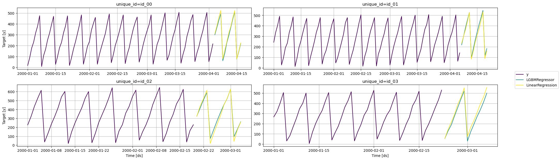 ## How to contribute See [CONTRIBUTING.md](https://github.com/Nixtla/mlforecast/blob/main/CONTRIBUTING.md). # Lag transforms Source: https://nixtlaverse.nixtla.io/mlforecast/lag_transforms.html Built-in lag transformations ## The `mlforecast.lag_transforms` module provides built-in **lag transformations**: statistics computed over lagged values of the target that are used as features by the forecasting model. You pass them to `MLForecast` through the `lag_transforms` argument, a dict whose keys are the lags to apply the transformation to and whose values are lists of transformation instances. ```python theme={null} from mlforecast import MLForecast from mlforecast.lag_transforms import ExpandingStd, RollingMean fcst = MLForecast( models=[...], freq='D', lag_transforms={ 1: [ExpandingStd()], 7: [RollingMean(window_size=7), RollingMean(window_size=28)], }, ) ``` The transforms fall into four families, each with several variants: * **Rolling** — `RollingMean`, `RollingStd`, `RollingMin`, `RollingMax`, `RollingQuantile`: fixed-window statistics over the lagged target. * **Seasonal rolling** — `SeasonalRollingMean`, `SeasonalRollingStd`, `SeasonalRollingMin`, `SeasonalRollingMax`, `SeasonalRollingQuantile`: rolling statistics computed across same-position observations in successive seasons (e.g. last 4 Mondays). * **Expanding** — `ExpandingMean`, `ExpandingStd`, `ExpandingMin`, `ExpandingMax`, `ExpandingQuantile`: statistics over all observations up to the lag. * **Exponentially weighted** — `ExponentiallyWeightedMean`: a weighted mean that emphasises recent observations. Two combinators let you build richer features from these primitives: **`Offset`** applies a transformation at a shifted lag, and **`Combine`** joins two transformations with a binary operator (for example a ratio of two rolling means at different windows). The basic usage is per-series — each transformation is computed independently for every series. The next section describes how to instead compute these statistics **across multiple series at once**. For a worked walkthrough of all of the above, including the `Combine` / `Offset` combinators and how to plug in custom numba-based transforms, see the [Lag transformations](docs/how-to-guides/lag_transforms_guide.html) how-to guide. ## Pooled mode: `global_`, `groupby`, and `partition_by` Every built-in rolling, expanding, seasonal-rolling, and exponentially weighted transform accepts three pooling parameters that let you compute the statistic across **multiple series at once**: * **`global_: bool`** — when `True`, the statistic is computed across **all series** aggregated by timestamp. Every series receives the same feature value at each timestamp. * **`groupby: Sequence[str]`** — column names to group by before computing the statistic. Columns must be declared as static features when calling `fit` / `preprocess`. Series in the same group share the feature value at each timestamp; series in different groups get different values. * **`partition_by: Sequence[str]`** — column names to partition further along a **dynamic** (time-varying) key, such as `promo` or `regime`. Each unique combination of partition values gets its own bucket. Composes with `global_` (cross-series aggregates within each partition), with `groupby` (group aggregates within each partition), or stands alone (per-(id, partition) buckets — *local* mode). Partition columns must be supplied via `X_df` at prediction. `global_` and `groupby` are **mutually exclusive** on the same transform. `partition_by` composes with either one or stands alone. All pooled modes require every series to **end at the same timestamp**, including local `partition_by`. **RANGE semantics.** Pooled transforms use SQL-style `RANGE BETWEEN ... PRECEDING` windows over actual timestamps, not row positions. Series with staggered starts simply do not contribute to the window until they have observations — no synthetic zeros are injected. Pooled mode assumes a **continuous, gap-free time grid** within each series; combining `validate_data=False` with a pooled transform raises a `UserWarning`. For `partition_by`, ordinals come from the **parent calendar** (global or group scope for nonlocal modes, per-id for local mode), so a partition bucket with gaps still preserves RANGE window semantics across those gaps rather than collapsing to row-based behavior. **`min_samples` divergence.** In local (per-series) mode, `min_samples` is capped at `window_size` by `coreforecast`. In pooled mode, `min_samples` counts **total non-NaN observations across all series** in the bucket within the rolling window, with no capping. This makes it useful as a coverage threshold: `RollingMean(window_size=1, min_samples=2, groupby=["brand"])` produces a non-null value only at timestamps where at least two series in the brand contribute observations. See the [Pooled lag transforms](docs/how-to-guides/pooled_lag_transforms.html) how-to guide for end-to-end examples. ### `RollingQuantile` ```python theme={null} RollingQuantile(p, window_size, min_samples=None, global_=False, groupby=None, partition_by=None, time_agg=None, **kwargs) ``` Bases:[\_RollingBase](#mlforecast.lag_transforms._RollingBase)
Rolling quantile.
[\_RollingBase](#mlforecast.lag_transforms._RollingBase)
Rolling statistic
### `RollingMin`
Bases: [\_RollingBase](#mlforecast.lag_transforms._RollingBase)
Rolling statistic
### `RollingStd`
Bases: [\_RollingBase](#mlforecast.lag_transforms._RollingBase)
Rolling statistic
### `RollingMean`
Bases: [\_RollingBase](#mlforecast.lag_transforms._RollingBase)
Rolling statistic
### `SeasonalRollingQuantile`
```python theme={null}
SeasonalRollingQuantile(p, season_length, window_size, min_samples=None, global_=False, groupby=None, partition_by=None, time_agg=None, **kwargs)
```
Bases: [\_Seasonal\_RollingBase](#mlforecast.lag_transforms._Seasonal_RollingBase)
Rolling statistic over seasonal periods
[\_Seasonal\_RollingBase](#mlforecast.lag_transforms._Seasonal_RollingBase)
Rolling statistic over seasonal periods
[\_Seasonal\_RollingBase](#mlforecast.lag_transforms._Seasonal_RollingBase)
Rolling statistic over seasonal periods
[\_Seasonal\_RollingBase](#mlforecast.lag_transforms._Seasonal_RollingBase)
Rolling statistic over seasonal periods
[\_Seasonal\_RollingBase](#mlforecast.lag_transforms._Seasonal_RollingBase)
Rolling statistic over seasonal periods
[\_ExpandingBase](#mlforecast.lag_transforms._ExpandingBase)
Expanding quantile.
[\_ExpandingBase](#mlforecast.lag_transforms._ExpandingBase)
Expanding statistic
**Parameters:**
| Name | Type | Description | Default |
| -------------- | --------------------------- | ----------------------------------------------------------------------------------------------------------------------------------------------------------------------------------------------------------------------------------------------------------------------------------------------------------------------------------------------------------------------------------------------------------------------------------------------------------------------- | ---------- |
| `global_` | bool | If True, compute the statistic across all series aggregated by timestamp. Requires all series to end at the same timestamp. Defaults to False. | *required* |
| `groupby` | Sequence\[str] | Column names to group by before computing the statistic. Columns must be static features. Mutually exclusive with `global_`. Defaults to None. | *required* |
| `partition_by` | Sequence\[str] | Column names to partition by. Each unique combination of partition values creates a separate bucket. Unlike `groupby`, partition columns may vary over time and must be supplied via `X_df` at prediction. Composes with `global_` (cross-series aggregates within each partition), `groupby` (group aggregates within each partition), or stands alone (per-(id, partition) buckets, *local* mode). See the Pooled lag transforms guide for details. Defaults to None. | *required* |
| `time_agg` | str | Pre-aggregate all rows sharing a timestamp within each bucket into a single value before applying the transform. One of `"sum"`, `"count"`, `"mean"`, `"min"`, `"max"`. Requires `global_` or `groupby`. Defaults to None. | *required* |
### `ExpandingMin`
Bases: [\_ExpandingBase](#mlforecast.lag_transforms._ExpandingBase)
Expanding statistic
**Parameters:**
| Name | Type | Description | Default |
| -------------- | --------------------------- | ----------------------------------------------------------------------------------------------------------------------------------------------------------------------------------------------------------------------------------------------------------------------------------------------------------------------------------------------------------------------------------------------------------------------------------------------------------------------- | ---------- |
| `global_` | bool | If True, compute the statistic across all series aggregated by timestamp. Requires all series to end at the same timestamp. Defaults to False. | *required* |
| `groupby` | Sequence\[str] | Column names to group by before computing the statistic. Columns must be static features. Mutually exclusive with `global_`. Defaults to None. | *required* |
| `partition_by` | Sequence\[str] | Column names to partition by. Each unique combination of partition values creates a separate bucket. Unlike `groupby`, partition columns may vary over time and must be supplied via `X_df` at prediction. Composes with `global_` (cross-series aggregates within each partition), `groupby` (group aggregates within each partition), or stands alone (per-(id, partition) buckets, *local* mode). See the Pooled lag transforms guide for details. Defaults to None. | *required* |
| `time_agg` | str | Pre-aggregate all rows sharing a timestamp within each bucket into a single value before applying the transform. One of `"sum"`, `"count"`, `"mean"`, `"min"`, `"max"`. Requires `global_` or `groupby`. Defaults to None. | *required* |
### `ExpandingStd`
Bases: [\_ExpandingBase](#mlforecast.lag_transforms._ExpandingBase)
Expanding statistic
**Parameters:**
| Name | Type | Description | Default |
| -------------- | --------------------------- | ----------------------------------------------------------------------------------------------------------------------------------------------------------------------------------------------------------------------------------------------------------------------------------------------------------------------------------------------------------------------------------------------------------------------------------------------------------------------- | ---------- |
| `global_` | bool | If True, compute the statistic across all series aggregated by timestamp. Requires all series to end at the same timestamp. Defaults to False. | *required* |
| `groupby` | Sequence\[str] | Column names to group by before computing the statistic. Columns must be static features. Mutually exclusive with `global_`. Defaults to None. | *required* |
| `partition_by` | Sequence\[str] | Column names to partition by. Each unique combination of partition values creates a separate bucket. Unlike `groupby`, partition columns may vary over time and must be supplied via `X_df` at prediction. Composes with `global_` (cross-series aggregates within each partition), `groupby` (group aggregates within each partition), or stands alone (per-(id, partition) buckets, *local* mode). See the Pooled lag transforms guide for details. Defaults to None. | *required* |
| `time_agg` | str | Pre-aggregate all rows sharing a timestamp within each bucket into a single value before applying the transform. One of `"sum"`, `"count"`, `"mean"`, `"min"`, `"max"`. Requires `global_` or `groupby`. Defaults to None. | *required* |
### `ExpandingMean`
Bases: [\_ExpandingBase](#mlforecast.lag_transforms._ExpandingBase)
Expanding statistic
**Parameters:**
| Name | Type | Description | Default |
| -------------- | --------------------------- | ----------------------------------------------------------------------------------------------------------------------------------------------------------------------------------------------------------------------------------------------------------------------------------------------------------------------------------------------------------------------------------------------------------------------------------------------------------------------- | ---------- |
| `global_` | bool | If True, compute the statistic across all series aggregated by timestamp. Requires all series to end at the same timestamp. Defaults to False. | *required* |
| `groupby` | Sequence\[str] | Column names to group by before computing the statistic. Columns must be static features. Mutually exclusive with `global_`. Defaults to None. | *required* |
| `partition_by` | Sequence\[str] | Column names to partition by. Each unique combination of partition values creates a separate bucket. Unlike `groupby`, partition columns may vary over time and must be supplied via `X_df` at prediction. Composes with `global_` (cross-series aggregates within each partition), `groupby` (group aggregates within each partition), or stands alone (per-(id, partition) buckets, *local* mode). See the Pooled lag transforms guide for details. Defaults to None. | *required* |
| `time_agg` | str | Pre-aggregate all rows sharing a timestamp within each bucket into a single value before applying the transform. One of `"sum"`, `"count"`, `"mean"`, `"min"`, `"max"`. Requires `global_` or `groupby`. Defaults to None. | *required* |
### `ExponentiallyWeightedMean`
```python theme={null}
ExponentiallyWeightedMean(alpha, global_=False, groupby=None, partition_by=None, time_agg='mean', **kwargs)
```
Bases: [\_BaseLagTransform](#mlforecast.lag_transforms._BaseLagTransform)
Exponentially weighted average
**Parameters:**
| Name | Type | Description | Default |
| -------------- | ------------------------------------------------------- | ----------------------------------------------------------------------------------------------------------------------------------------------------------------------------------------------------------------------------------------------------------------------------------------------------------------------------------------------------------------------------------------------------------------------------------------------------------------------- | ------------------- |
| `alpha` | [float](#float) | Smoothing factor. | *required* |
| `global_` | [bool](#bool) | If True, compute the statistic across all series aggregated by timestamp. Requires all series to end at the same timestamp. Defaults to False. | False |
| `groupby` | [Sequence](#typing.Sequence)\[[str](#str)] | Column names to group by before computing the statistic. Columns must be static features. Mutually exclusive with `global_`. Defaults to None. | None |
| `partition_by` | [Sequence](#typing.Sequence)\[[str](#str)] | Column names to partition by. Each unique combination of partition values creates a separate bucket. Unlike `groupby`, partition columns may vary over time and must be supplied via `X_df` at prediction. Composes with `global_` (cross-series aggregates within each partition), `groupby` (group aggregates within each partition), or stands alone (per-(id, partition) buckets, *local* mode). See the Pooled lag transforms guide for details. Defaults to None. | None |
| `time_agg` | [str](#str) | Pre-aggregate all rows sharing a timestamp within each bucket into a single value before applying the transform. One of `"sum"`, `"count"`, `"mean"`, `"min"`, `"max"`. Values other than `"mean"` require `global_` or `groupby`. Defaults to `"mean"`, which matches EWM's bucket-mean update rule: each timestamp contributes its bucket aggregate mean exactly once, regardless of how many rows aggregated there. `None` is not accepted. | 'mean' |
### `Offset`
```python theme={null}
Offset(tfm, n)
```
Bases: [\_BaseLagTransform](#mlforecast.lag_transforms._BaseLagTransform)
Shift series before computing transformation
**Parameters:**
| Name | Type | Description | Default |
| ----- | ------------------------------------------ | ---------------------------------------------------------------------------- | ---------- |
| `tfm` | [LagTransform](#LagTransform) | Transformation to be applied | *required* |
| `n` | [int](#int) | Number of positions to shift (lag) series before applying the transformation | *required* |
### `Combine`
```python theme={null}
Combine(tfm1, tfm2, operator)
```
Bases: [\_BaseLagTransform](#mlforecast.lag_transforms._BaseLagTransform)
Combine two lag transformations using an operator
**Parameters:**
| Name | Type | Description | Default |
| ---------- | ------------------------------------------ | -------------------------------------------------------------------- | ---------- |
| `tfm1` | [LagTransform](#LagTransform) | First transformation. | *required* |
| `tfm2` | [LagTransform](#LagTransform) | Second transformation. | *required* |
| `operator` | [callable](#callable) | Binary operator that defines how to combine the two transformations. | *required* |
# LightGBMCV
Source: https://nixtlaverse.nixtla.io/mlforecast/lgb_cv.html
Time series cross validation with LightGBM.
##
### `LightGBMCV`
```python theme={null}
LightGBMCV(freq, lags=None, lag_transforms=None, date_features=None, num_threads=1, target_transforms=None)
```
Create LightGBM CV object.
**Parameters:**
| Name | Type | Description | Default |
| ------------------- | --------------------------------------------- | ------------------------------------------------------------------------------------------------------------------------------------------- | ----------------- |
| `freq` | [str](#str) or [int](#int) | Pandas offset alias, e.g. 'D', 'W-THU' or integer denoting the frequency of the series. | *required* |
| `lags` | list of int | Lags of the target to use as features. Defaults to None. | None |
| `lag_transforms` | dict of int to list of functions | Mapping of target lags to their transformations. Defaults to None. | None |
| `date_features` | list of str or callable | Features computed from the dates. Can be pandas date attributes or functions that will take the dates as input. Defaults to None. | None |
| `num_threads` | [int](#int) | Number of threads to use when computing the features. Use -1 to use all available CPU cores. Defaults to 1. | 1 |
| `target_transforms` | list of transformers | Transformations that will be applied to the target before computing the features and restored after the forecasting step. Defaults to None. | None |
#### `LightGBMCV.fit`
```python theme={null}
fit(df, n_windows, h, id_col='unique_id', time_col='ds', target_col='y', step_size=None, num_iterations=100, params=None, static_features=None, dropna=True, keep_last_n=None, eval_every=10, weights=None, metric='mape', verbose_eval=True, early_stopping_evals=2, early_stopping_pct=0.01, compute_cv_preds=False, before_predict_callback=None, after_predict_callback=None, input_size=None, weight_col=None)
```
Train boosters simultaneously and assess their performance on the complete forecasting window.
**Parameters:**
| Name | Type | Description | Default |
| ------------------------- | ------------------------------------------------- | ------------------------------------------------------------------------------------------------------------------------------------------------------------------------------------------------------------------------------------------------------------------------------------------------------------------------------------------- | ------------------------- |
| `df` | pandas DataFrame | Series data in long format. | *required* |
| `n_windows` | [int](#int) | Number of windows to evaluate. | *required* |
| `h` | [int](#int) | Forecast horizon. | *required* |
| `id_col` | [str](#str) | Column that identifies each serie. Defaults to 'unique\_id'. | 'unique\_id' |
| `time_col` | [str](#str) | Column that identifies each timestep, its values can be timestamps or integers. Defaults to 'ds'. | 'ds' |
| `target_col` | [str](#str) | Column that contains the target. Defaults to 'y'. | 'y' |
| `step_size` | [int](#int) | Step size between each cross validation window. If None it will be equal to `h`. Defaults to None. | None |
| `num_iterations` | [int](#int) | Maximum number of boosting iterations to run. Defaults to 100. | 100 |
| `params` | [dict](#dict) | Parameters to be passed to the LightGBM Boosters. Defaults to None. | None |
| `static_features` | list of str | Names of the features that are static and will be repeated when forecasting. Defaults to None. | None |
| `dropna` | [bool](#bool) | Drop rows with missing values produced by the transformations. Defaults to True. | True |
| `keep_last_n` | [int](#int) | Keep only these many records from each serie for the forecasting step. Can save time and memory if your features allow it. Pooled lag transforms (global\_/groupby/partition\_by) with a window wider than this keep that wider window instead, since their shared aggregates have no per-series buffer to trim below it. Defaults to None. | None |
| `eval_every` | [int](#int) | Number of boosting iterations to train before evaluating on the whole forecast window. Defaults to 10. | 10 |
| `weights` | sequence of float | Weights to multiply the metric of each window. If None, all windows have the same weight. Defaults to None. | None |
| `metric` | [str](#str) or [callable](#callable) | Metric used to assess the performance of the models and perform early stopping. Defaults to 'mape'. | 'mape' |
| `verbose_eval` | [bool](#bool) | Print the metrics of each evaluation. | True |
| `early_stopping_evals` | [int](#int) | Maximum number of evaluations to run without improvement. Defaults to 2. | 2 |
| `early_stopping_pct` | [float](#float) | Minimum percentage improvement in metric value in `early_stopping_evals` evaluations. Defaults to 0.01. | 0.01 |
| `compute_cv_preds` | [bool](#bool) | Compute predictions for each window after finding the best iteration. Defaults to False. | False |
| `before_predict_callback` | [callable](#callable) | Function to call on the features before computing the predictions. This function will take the input dataframe that will be passed to the model for predicting and should return a dataframe with the same structure. The series identifier is on the index. Defaults to None. | None |
| `after_predict_callback` | [callable](#callable) | Function to call on the predictions before updating the targets. This function will take a pandas Series with the predictions and should return another one with the same structure. The series identifier is on the index. Defaults to None. | None |
| `input_size` | [int](#int) | Maximum training samples per serie in each window. If None, will use an expanding window. Defaults to None. | None |
**Returns:**
| Type | Description |
| -------------------------- | ----------------------------------------------- |
| list of tuple | List of (boosting rounds, metric value) tuples. |
#### `LightGBMCV.predict`
```python theme={null}
predict(h, before_predict_callback=None, after_predict_callback=None, X_df=None)
```
Compute predictions with each of the trained boosters.
**Parameters:**
| Name | Type | Description | Default |
| ------------------------- | ------------------------------------------- | ------------------------------------------------------------------------------------------------------------------------------------------------------------------------------------------------------------------------------------------------------------------------------ | ----------------- |
| `h` | [int](#int) | Forecast horizon. | *required* |
| `before_predict_callback` | [callable](#callable) | Function to call on the features before computing the predictions. This function will take the input dataframe that will be passed to the model for predicting and should return a dataframe with the same structure. The series identifier is on the index. Defaults to None. | None |
| `after_predict_callback` | [callable](#callable) | Function to call on the predictions before updating the targets. This function will take a pandas Series with the predictions and should return another one with the same structure. The series identifier is on the index. Defaults to None. | None |
| `X_df` | [DataFrame](#pandas.DataFrame) | Dataframe with the future exogenous features. Should have the id column and the time column. Defaults to None. | None |
**Returns:**
| Type | Description |
| ------------------------------------------- | -------------------------------------------------------------------- |
| [DataFrame](#pandas.DataFrame) | Predictions for each serie and timestep, with one column per window. |
#### `LightGBMCV.setup`
```python theme={null}
setup(df, n_windows, h, id_col='unique_id', time_col='ds', target_col='y', step_size=None, params=None, static_features=None, dropna=True, keep_last_n=None, weights=None, metric='mape', input_size=None, weight_col=None)
```
Initialize internal data structures to iteratively train the boosters. Use this before calling partial\_fit.
**Parameters:**
| Name | Type | Description | Default |
| ----------------- | ------------------------------------------------- | ------------------------------------------------------------------------------------------------------------------------------------------------------------------------------------------------------------------------------------------------------------------------------------------------------------------------------------------- | ------------------------- |
| `df` | pandas DataFrame | Series data in long format. | *required* |
| `n_windows` | [int](#int) | Number of windows to evaluate. | *required* |
| `h` | [int](#int) | Forecast horizon. | *required* |
| `id_col` | [str](#str) | Column that identifies each serie. Defaults to 'unique\_id'. | 'unique\_id' |
| `time_col` | [str](#str) | Column that identifies each timestep, its values can be timestamps or integers. Defaults to 'ds'. | 'ds' |
| `target_col` | [str](#str) | Column that contains the target. Defaults to 'y'. | 'y' |
| `step_size` | [int](#int) | Step size between each cross validation window. If None it will be equal to `h`. Defaults to None. | None |
| `params` | [dict](#dict) | Parameters to be passed to the LightGBM Boosters. Defaults to None. | None |
| `static_features` | list of str | Names of the features that are static and will be repeated when forecasting. Defaults to None. | None |
| `dropna` | [bool](#bool) | Drop rows with missing values produced by the transformations. Defaults to True. | True |
| `keep_last_n` | [int](#int) | Keep only these many records from each serie for the forecasting step. Can save time and memory if your features allow it. Pooled lag transforms (global\_/groupby/partition\_by) with a window wider than this keep that wider window instead, since their shared aggregates have no per-series buffer to trim below it. Defaults to None. | None |
| `weights` | sequence of float | Weights to multiply the metric of each window. If None, all windows have the same weight. Defaults to None. | None |
| `metric` | [str](#str) or [callable](#callable) | Metric used to assess the performance of the models and perform early stopping. Defaults to 'mape'. | 'mape' |
| `input_size` | [int](#int) | Maximum training samples per serie in each window. If None, will use an expanding window. Defaults to None. | None |
| `weight_col` | [str](#str) | Column containing sample weights. Higher weights increase the influence of those samples during fitting and evaluation. | None |
**Returns:**
| Type | Description |
| -------------------------------------------------------- | --------------------------------------------------------- |
| [LightGBMCV](#mlforecast.lgb_cv.LightGBMCV) | CV object with internal data structures for partial\_fit. |
#### `LightGBMCV.partial_fit`
```python theme={null}
partial_fit(num_iterations, before_predict_callback=None, after_predict_callback=None, weight_col=None)
```
Train the boosters for some iterations.
**Parameters:**
| Name | Type | Description | Default |
| ------------------------- | ---------------------------------- | ------------------------------------------------------------------------------------------------------------------------------------------------------------------------------------------------------------------------------------------------------------------------------ | ----------------- |
| `num_iterations` | [int](#int) | Number of boosting iterations to run | *required* |
| `before_predict_callback` | [callable](#callable) | Function to call on the features before computing the predictions. This function will take the input dataframe that will be passed to the model for predicting and should return a dataframe with the same structure. The series identifier is on the index. Defaults to None. | None |
| `after_predict_callback` | [callable](#callable) | Function to call on the predictions before updating the targets. This function will take a pandas Series with the predictions and should return another one with the same structure. The series identifier is on the index. Defaults to None. | None |
**Returns:**
| Type | Description |
| ---------------------------- | --------------------------------------------------- |
| [float](#float) | Weighted metric after training for num\_iterations. |
### Example
This shows an example with just 4 series of the M4 dataset. If you want
to run it yourself on all of them, you can refer to [this
notebook](https://www.kaggle.com/code/lemuz90/m4-competition-cv).
```python theme={null}
import random
from datasetsforecast.m4 import M4, M4Info
from fastcore.test import test_eq, test_fail
from mlforecast.target_transforms import Differences
from nbdev import show_doc
from mlforecast.lag_transforms import SeasonalRollingMean
```
```python theme={null}
group = 'Hourly'
await M4.async_download('data', group=group)
df, *_ = M4.load(directory='data', group=group)
df['ds'] = df['ds'].astype('int')
ids = df['unique_id'].unique()
random.seed(0)
sample_ids = random.choices(ids, k=4)
sample_df = df[df['unique_id'].isin(sample_ids)]
sample_df
```
| | unique\_id | ds | y |
| ------ | ---------- | ---- | ---- |
| 86796 | H196 | 1 | 11.8 |
| 86797 | H196 | 2 | 11.4 |
| 86798 | H196 | 3 | 11.1 |
| 86799 | H196 | 4 | 10.8 |
| 86800 | H196 | 5 | 10.6 |
| ... | ... | ... | ... |
| 325235 | H413 | 1004 | 99.0 |
| 325236 | H413 | 1005 | 88.0 |
| 325237 | H413 | 1006 | 47.0 |
| 325238 | H413 | 1007 | 41.0 |
| 325239 | H413 | 1008 | 34.0 |
```python theme={null}
info = M4Info[group]
horizon = info.horizon
valid = sample_df.groupby('unique_id').tail(horizon)
train = sample_df.drop(valid.index)
train.shape, valid.shape
```
```text theme={null}
((3840, 3), (192, 3))
```
What LightGBMCV does is emulate [LightGBM’s cv
function](https://lightgbm.readthedocs.io/en/v3.3.2/pythonapi/lightgbm.cv.html#lightgbm.cv)
where several Boosters are trained simultaneously on different
partitions of the data, that is, one boosting iteration is performed on
all of them at a time. This allows to have an estimate of the error by
iteration, so if we combine this with early stopping we can find the
best iteration to train a final model using all the data or even use
these individual models’ predictions to compute an ensemble.
In order to have a good estimate of the forecasting performance of our
model we compute predictions for the whole test period and compute a
metric on that. Since this step can slow down training, there’s an
`eval_every` parameter that can be used to control this, that is, if
`eval_every=10` (the default) every 10 boosting iterations we’re going
to compute forecasts for the complete window and report the error.
We also have early stopping parameters:
* `early_stopping_evals`: how many evaluations of the full window
should we go without improving to stop training?
* `early_stopping_pct`: what’s the minimum percentage improvement we
want in these `early_stopping_evals` in order to keep training?
This makes the LightGBMCV class a good tool to quickly test different
configurations of the model. Consider the following example, where we’re
going to try to find out which features can improve the performance of
our model. We start just using lags.
```python theme={null}
static_fit_config = dict(
n_windows=2,
h=horizon,
params={'verbose': -1},
compute_cv_preds=True,
)
cv = LightGBMCV(
freq=1,
lags=[24 * (i+1) for i in range(7)], # one week of lags
)
```
```python theme={null}
hist = cv.fit(train, **static_fit_config)
```
```text theme={null}
[LightGBM] [Info] Start training from score 51.745632
[10] mape: 0.590690
[20] mape: 0.251093
[30] mape: 0.143643
[40] mape: 0.109723
[50] mape: 0.102099
[60] mape: 0.099448
[70] mape: 0.098349
[80] mape: 0.098006
[90] mape: 0.098718
Early stopping at round 90
Using best iteration: 80
```
By setting `compute_cv_preds` we get the predictions from each model on
their corresponding validation fold.
```python theme={null}
cv.cv_preds_
```
| | unique\_id | ds | y | Booster | window |
| --- | ---------- | --- | ---- | --------- | ------ |
| 0 | H196 | 865 | 15.5 | 15.522924 | 0 |
| 1 | H196 | 866 | 15.1 | 14.985832 | 0 |
| 2 | H196 | 867 | 14.8 | 14.667901 | 0 |
| 3 | H196 | 868 | 14.4 | 14.514592 | 0 |
| 4 | H196 | 869 | 14.2 | 14.035793 | 0 |
| ... | ... | ... | ... | ... | ... |
| 187 | H413 | 956 | 59.0 | 77.227905 | 1 |
| 188 | H413 | 957 | 58.0 | 80.589641 | 1 |
| 189 | H413 | 958 | 53.0 | 53.986834 | 1 |
| 190 | H413 | 959 | 38.0 | 36.749786 | 1 |
| 191 | H413 | 960 | 46.0 | 36.281225 | 1 |
The individual models we trained are saved, so calling `predict` returns
the predictions from every model trained.
```python theme={null}
preds = cv.predict(horizon)
preds
```
| | unique\_id | ds | Booster0 | Booster1 |
| --- | ---------- | ---- | --------- | --------- |
| 0 | H196 | 961 | 15.670252 | 15.848888 |
| 1 | H196 | 962 | 15.522924 | 15.697399 |
| 2 | H196 | 963 | 14.985832 | 15.166213 |
| 3 | H196 | 964 | 14.985832 | 14.723238 |
| 4 | H196 | 965 | 14.562152 | 14.451092 |
| ... | ... | ... | ... | ... |
| 187 | H413 | 1004 | 70.695242 | 65.917620 |
| 188 | H413 | 1005 | 66.216580 | 62.615788 |
| 189 | H413 | 1006 | 63.896573 | 67.848598 |
| 190 | H413 | 1007 | 46.922797 | 50.981950 |
| 191 | H413 | 1008 | 45.006541 | 42.752819 |
We can average these predictions and evaluate them.
```python theme={null}
def evaluate_on_valid(preds):
preds = preds.copy()
preds['final_prediction'] = preds.drop(columns=['unique_id', 'ds']).mean(1)
merged = preds.merge(valid, on=['unique_id', 'ds'])
merged['abs_err'] = abs(merged['final_prediction'] - merged['y']) / merged['y']
return merged.groupby('unique_id')['abs_err'].mean().mean()
```
```python theme={null}
eval1 = evaluate_on_valid(preds)
eval1
```
```text theme={null}
0.11036194712311806
```
Now, since these series are hourly, maybe we can try to remove the daily
seasonality by taking the 168th (24 \* 7) difference, that is, substract
the value at the same hour from one week ago, thus our target will be
$z_t = y_{t} - y_{t-168}$. The features will be computed from this
target and when we predict they will be automatically re-applied.
```python theme={null}
cv2 = LightGBMCV(
freq=1,
target_transforms=[Differences([24 * 7])],
lags=[24 * (i+1) for i in range(7)],
)
hist2 = cv2.fit(train, **static_fit_config)
```
```text theme={null}
[LightGBM] [Info] Start training from score 0.519010
[10] mape: 0.089024
[20] mape: 0.090683
[30] mape: 0.092316
Early stopping at round 30
Using best iteration: 10
```
```python theme={null}
assert hist2[-1][1] < hist[-1][1]
```
Nice! We achieve a better score in less iterations. Let’s see if this
improvement translates to the validation set as well.
```python theme={null}
preds2 = cv2.predict(horizon)
eval2 = evaluate_on_valid(preds2)
eval2
```
```text theme={null}
0.08956665504570135
```
```python theme={null}
assert eval2 < eval1
```
Great! Maybe we can try some lag transforms now. We’ll try the seasonal
rolling mean that averages the values “every season”, that is, if we set
`season_length=24` and `window_size=7` then we’ll average the value at
the same hour for every day of the week.
```python theme={null}
cv3 = LightGBMCV(
freq=1,
target_transforms=[Differences([24 * 7])],
lags=[24 * (i+1) for i in range(7)],
lag_transforms={
48: [SeasonalRollingMean(season_length=24, window_size=7)],
},
)
hist3 = cv3.fit(train, **static_fit_config)
```
```text theme={null}
[LightGBM] [Info] Start training from score 0.273641
[10] mape: 0.086724
[20] mape: 0.088466
[30] mape: 0.090536
Early stopping at round 30
Using best iteration: 10
```
Seems like this is helping as well!
```python theme={null}
assert hist3[-1][1] < hist2[-1][1]
```
Does this reflect on the validation set?
```python theme={null}
preds3 = cv3.predict(horizon)
eval3 = evaluate_on_valid(preds3)
eval3
```
```text theme={null}
0.08961279023129345
```
Nice! mlforecast also supports date features, but in this case our time
column is made from integers so there aren’t many possibilites here. As
you can see this allows you to iterate faster and get better estimates
of the forecasting performance you can expect from your model.
If you’re doing hyperparameter tuning it’s useful to be able to run a
couple of iterations, assess the performance, and determine if this
particular configuration isn’t promising and should be discarded. For
example, [optuna](https://optuna.org/) has
[pruners](https://optuna.readthedocs.io/en/stable/reference/pruners.html)
that you can call with your current score and it decides if the trial
should be discarded. We’ll now show how to do that.
Since the CV requires a bit of setup, like the LightGBM datasets and the
internal features, we have this `setup` method.
```python theme={null}
cv4 = LightGBMCV(
freq=1,
lags=[24 * (i+1) for i in range(7)],
)
cv4.setup(
train,
n_windows=2,
h=horizon,
params={'verbose': -1},
)
```
```text theme={null}
LightGBMCV(freq=1, lag_features=['lag24', 'lag48', 'lag72', 'lag96', 'lag120', 'lag144', 'lag168'], date_features=[], num_threads=1, bst_threads=8)
```
Once we have this we can call `partial_fit` to only train for some
iterations and return the score of the forecast window.
```python theme={null}
score = cv4.partial_fit(10)
score
```
```text theme={null}
[LightGBM] [Info] Start training from score 51.745632
```
```text theme={null}
0.5906900462828166
```
This is equal to the first evaluation from our first example.
```python theme={null}
assert hist[0][1] == score
```
We can now use this score to decide if this configuration is promising.
If we want to we can train some more iterations.
```python theme={null}
score2 = cv4.partial_fit(20)
```
This is now equal to our third metric from the first example, since this
time we trained for 20 iterations.
```python theme={null}
assert hist[2][1] == score2
```
### Using a custom metric
The built-in metrics are MAPE and RMSE, which are computed by serie and
then averaged across all series. If you want to do something different
or use a different metric entirely, you can define your own metric like
the following:
```python theme={null}
def weighted_mape(
y_true: pd.Series,
y_pred: pd.Series,
ids: pd.Series,
dates: pd.Series,
):
"""Weighs the MAPE by the magnitude of the series values"""
abs_pct_err = abs(y_true - y_pred) / abs(y_true)
mape_by_serie = abs_pct_err.groupby(ids).mean()
totals_per_serie = y_pred.groupby(ids).sum()
series_weights = totals_per_serie / totals_per_serie.sum()
return (mape_by_serie * series_weights).sum()
```
```python theme={null}
_ = LightGBMCV(
freq=1,
lags=[24 * (i+1) for i in range(7)],
).fit(
train,
n_windows=2,
h=horizon,
params={'verbose': -1},
metric=weighted_mape,
)
```
```text theme={null}
[LightGBM] [Info] Start training from score 51.745632
[10] weighted_mape: 0.480353
[20] weighted_mape: 0.218670
[30] weighted_mape: 0.161706
[40] weighted_mape: 0.149992
[50] weighted_mape: 0.149024
[60] weighted_mape: 0.148496
Early stopping at round 60
Using best iteration: 60
```
# Optimization
Source: https://nixtlaverse.nixtla.io/mlforecast/optimization.html
Utilities for hyperparameter optimization
##
### `mlforecast_objective`
```python theme={null}
mlforecast_objective(df, config_fn, loss, model, freq, n_windows, h, step_size=None, input_size=None, refit=False, id_col='unique_id', time_col='ds', target_col='y', weight_col=None, cv_splits=None)
```
optuna objective function for the MLForecast class
**Parameters:**
| Name | Type | Description | Default |
| ------------ | ------------------------------------------------------------------------------------------------------------------------------------------------------------------------------------------------------------- | --------------------------------------------------------------------------------------------------------------------------------------------------------------------------------------------------------------------------- | ------------------------- |
| `df` | [DataFrame](#utilsforecast.compat.DataFrame) | Series data in long format. | *required* |
| `config_fn` | [callable](#callable) | Function that takes an optuna trial and produces a configuration with the following keys: - model\_params - mlf\_init\_params - mlf\_fit\_params | *required* |
| `loss` | [callable](#callable) | Function that takes the validation and train dataframes and produces a float. | *required* |
| `model` | [BaseEstimator](#sklearn.base.BaseEstimator) | scikit-learn compatible model to be trained | *required* |
| `freq` | [str](#str) or [int](#int) | pandas' or polars' offset alias or integer denoting the frequency of the series. | *required* |
| `n_windows` | [int](#int) | Number of windows to evaluate. | *required* |
| `h` | [int](#int) | Forecast horizon. | *required* |
| `step_size` | [int](#int) | Step size between each cross validation window. If None it will be equal to `h`. Defaults to None. | None |
| `input_size` | [int](#int) | Maximum training samples per serie in each window. If None, will use an expanding window. Defaults to None. | None |
| `refit` | [bool](#bool) or [int](#int) | Retrain model for each cross validation window. If False, the models are trained at the beginning and then used to predict each window. If positive int, the models are retrained every `refit` windows. Defaults to False. | False |
| `id_col` | [str](#str) | Column that identifies each serie. Defaults to 'unique\_id'. | 'unique\_id' |
| `time_col` | [str](#str) | Column that identifies each timestep, its values can be timestamps or integers. Defaults to 'ds'. | 'ds' |
| `target_col` | [str](#str) | Column that contains the target. Defaults to 'y'. | 'y' |
| `weight_col` | [str](#str) | Column that contains sample weights. Defaults to None. | None |
| `cv_splits` | [List](#typing.List)\[[Tuple](#typing.Tuple)\[[DataFrame](#utilsforecast.compat.DataFrame), [DataFrame](#utilsforecast.compat.DataFrame), [DataFrame](#utilsforecast.compat.DataFrame)]] \| None | Optional cached CV splits (cutoffs, train, valid) to reuse across trials. If None, backtest splits are generated on each trial. | None |
**Returns:**
| Type | Description |
| -------------------------------------------------------------------------------------- | ------------------------- |
| [Callable](#typing.Callable)\[\[[Trial](#optuna.Trial)], [float](#float)] | optuna objective function |
```python theme={null}
import lightgbm as lgb
from datasetsforecast.m4 import M4, M4Evaluation, M4Info
from utilsforecast.losses import smape
from mlforecast.lag_transforms import ExpandingMean, RollingMean
from mlforecast.target_transforms import Differences, LocalBoxCox, LocalStandardScaler
```
```python theme={null}
def train_valid_split(group):
df, *_ = M4.load(directory='data', group=group)
df['ds'] = df['ds'].astype('int')
horizon = M4Info[group].horizon
valid = df.groupby('unique_id').tail(horizon)
train = df.drop(valid.index)
return train, valid
```
```python theme={null}
h = M4Info['Weekly'].horizon
weekly_train, weekly_valid = train_valid_split('Weekly')
weekly_train['unique_id'] = weekly_train['unique_id'].astype('category')
weekly_valid['unique_id'] = weekly_valid['unique_id'].astype(weekly_train['unique_id'].dtype)
```
```python theme={null}
def config_fn(trial):
candidate_lags = [
[1],
[13],
[1, 13],
range(1, 33),
]
lag_idx = trial.suggest_categorical('lag_idx', range(len(candidate_lags)))
candidate_lag_tfms = [
{
1: [RollingMean(window_size=13)]
},
{
1: [RollingMean(window_size=13)],
13: [RollingMean(window_size=13)],
},
{
13: [RollingMean(window_size=13)],
},
{
4: [ExpandingMean(), RollingMean(window_size=4)],
8: [ExpandingMean(), RollingMean(window_size=4)],
}
]
lag_tfms_idx = trial.suggest_categorical('lag_tfms_idx', range(len(candidate_lag_tfms)))
candidate_targ_tfms = [
[Differences([1])],
[LocalBoxCox()],
[LocalStandardScaler()],
[LocalBoxCox(), Differences([1])],
[LocalBoxCox(), LocalStandardScaler()],
[LocalBoxCox(), Differences([1]), LocalStandardScaler()],
]
targ_tfms_idx = trial.suggest_categorical('targ_tfms_idx', range(len(candidate_targ_tfms)))
return {
'model_params': {
'learning_rate': 0.05,
'objective': 'l1',
'bagging_freq': 1,
'num_threads': 2,
'verbose': -1,
'force_col_wise': True,
'n_estimators': trial.suggest_int('n_estimators', 10, 1000, log=True),
'num_leaves': trial.suggest_int('num_leaves', 31, 1024, log=True),
'lambda_l1': trial.suggest_float('lambda_l1', 0.01, 10, log=True),
'lambda_l2': trial.suggest_float('lambda_l2', 0.01, 10, log=True),
'bagging_fraction': trial.suggest_float('bagging_fraction', 0.75, 1.0),
'feature_fraction': trial.suggest_float('feature_fraction', 0.75, 1.0),
},
'mlf_init_params': {
'lags': candidate_lags[lag_idx],
'lag_transforms': candidate_lag_tfms[lag_tfms_idx],
'target_transforms': candidate_targ_tfms[targ_tfms_idx],
},
'mlf_fit_params': {
'static_features': ['unique_id'],
}
}
def loss(df, train_df):
return smape(df, models=['model'])['model'].mean()
```
```python theme={null}
optuna.logging.set_verbosity(optuna.logging.WARNING)
objective = mlforecast_objective(
df=weekly_train,
config_fn=config_fn,
loss=loss,
model=lgb.LGBMRegressor(),
freq=1,
n_windows=2,
h=h,
)
study = optuna.create_study(
direction='minimize', sampler=optuna.samplers.TPESampler(seed=0)
)
study.optimize(objective, n_trials=2)
best_cfg = study.best_trial.user_attrs['config']
final_model = MLForecast(
models=[lgb.LGBMRegressor(**best_cfg['model_params'])],
freq=1,
**best_cfg['mlf_init_params'],
)
final_model.fit(weekly_train, **best_cfg['mlf_fit_params'])
preds = final_model.predict(h)
M4Evaluation.evaluate('data', 'Weekly', preds['LGBMRegressor'].values.reshape(-1, 13))
```
| | SMAPE | MASE | OWA |
| ------ | -------- | -------- | -------- |
| Weekly | 9.261538 | 2.614473 | 0.976158 |
# Target transforms
Source: https://nixtlaverse.nixtla.io/mlforecast/target_transforms.html
##
```python theme={null}
import pandas as pd
from fastcore.test import test_fail
from sklearn.ensemble import HistGradientBoostingRegressor
from sklearn.linear_model import LinearRegression
from sklearn.preprocessing import PowerTransformer
from utilsforecast.processing import counts_by_id
from mlforecast import MLForecast
from mlforecast.utils import generate_daily_series
```
### `BaseTargetTransform`
Bases: [ABC](#abc.ABC)
Base class used for target transformations.
### `Differences`
```python theme={null}
Differences(differences)
```
Bases: [\_BaseGroupedArrayTargetTransform](#mlforecast.target_transforms._BaseGroupedArrayTargetTransform)
Subtracts previous values of the serie. Can be used to remove trend or seasonalities.
```python theme={null}
series = generate_daily_series(10, min_length=50, max_length=100)
diffs = Differences([1, 2, 5])
id_counts = counts_by_id(series, 'unique_id')
indptr = np.append(0, id_counts['counts'].cumsum())
ga = GroupedArray(series['y'].values, indptr)
# differences are applied correctly
transformed = diffs.fit_transform(ga)
assert diffs.fitted_ == []
expected = series.copy()
for d in diffs.differences:
expected['y'] -= expected.groupby('unique_id', observed=True)['y'].shift(d)
np.testing.assert_allclose(transformed.data, expected['y'].values)
# fitted differences are restored correctly
diffs.store_fitted = True
transformed = diffs.fit_transform(ga)
keep_mask = ~np.isnan(transformed.data)
restored = diffs.inverse_transform_fitted(transformed)
np.testing.assert_allclose(ga.data[keep_mask], restored.data[keep_mask])
# test transform
new_ga = GroupedArray(np.random.rand(10), np.arange(11))
prev_orig = [diffs.scalers_[i].tails_[::d].copy() for i, d in enumerate(diffs.differences)]
expected = new_ga.data - np.add.reduce(prev_orig)
updates = diffs.update(new_ga)
np.testing.assert_allclose(expected, updates.data)
np.testing.assert_allclose(diffs.scalers_[0].tails_, new_ga.data)
np.testing.assert_allclose(diffs.scalers_[1].tails_[1::2], new_ga.data - prev_orig[0])
np.testing.assert_allclose(diffs.scalers_[2].tails_[4::5], new_ga.data - np.add.reduce(prev_orig[:2]))
# variable sizes
diff1 = Differences([1])
ga = GroupedArray(np.arange(10), np.array([0, 3, 10]))
diff1.fit_transform(ga)
new_ga = GroupedArray(np.arange(4), np.array([0, 1, 4]))
updates = diff1.update(new_ga)
np.testing.assert_allclose(updates.data, np.array([0 - 2, 1 - 9, 2 - 1, 3 - 2]))
np.testing.assert_allclose(diff1.scalers_[0].tails_, np.array([0, 3]))
# short series
ga = GroupedArray(np.arange(20), np.array([0, 2, 20]))
test_fail(lambda: diffs.fit_transform(ga), contains="[0]")
# stack
diffs = Differences([1, 2, 5])
ga = GroupedArray(series['y'].values, indptr)
diffs.fit_transform(ga)
stacked = Differences.stack([diffs, diffs])
for i in range(len(diffs.differences)):
np.testing.assert_allclose(
stacked.scalers_[i].tails_,
np.tile(diffs.scalers_[i].tails_, 2)
)
```
### `AutoDifferences`
```python theme={null}
AutoDifferences(max_diffs)
```
Bases: [\_BaseGroupedArrayTargetTransform](#mlforecast.target_transforms._BaseGroupedArrayTargetTransform)
Find and apply the optimal number of differences to each serie.
**Parameters:**
| Name | Type | Description | Default |
| ----------- | ------------------------ | --------------------------------------- | ---------- |
| `max_diffs` | [int](#int) | Maximum number of differences to apply. | *required* |
#### `AutoDifferences.inverse_transform_fitted`
```python theme={null}
inverse_transform_fitted(ga)
```
Inverse transform fitted values.
Reverses the differencing transformation by reconstructing the original
values from the differenced fitted values. This is used when fitted=True
to restore the fitted predictions to the original scale.
**Parameters:**
| Name | Type | Description | Default |
| ---- | ------------------------------------------------------------------- | ------------------------------------------------------ | ---------- |
| `ga` | [GroupedArray](#mlforecast.grouped_array.GroupedArray) | GroupedArray containing the differenced fitted values. | *required* |
**Returns:**
| Type | Description |
| ------------------------------------------------------------------- | ------------------------------------------------------ |
| [GroupedArray](#mlforecast.grouped_array.GroupedArray) | GroupedArray with fitted values in the original scale. |
**Raises:**
| Type | Description |
| -------------------------------------- | ------------------------------------------------------- |
| [ValueError](#ValueError) | If fitted differences are smaller than provided target. |
### `AutoSeasonalDifferences`
```python theme={null}
AutoSeasonalDifferences(season_length, max_diffs, n_seasons=10)
```
Bases: [AutoDifferences](#mlforecast.target_transforms.AutoDifferences)
Find and apply the optimal number of seasonal differences to each group.
**Parameters:**
| Name | Type | Description | Default |
| --------------- | ------------------------ | ------------------------------------------------------------------------------------------------------------------------------------------------------------------------------------------------------------------------------------------------------ | --------------- |
| `season_length` | [int](#int) | Length of the seasonal period. | *required* |
| `max_diffs` | [int](#int) | Maximum number of differences to apply. | *required* |
| `n_seasons` | [int](#int) | Number of seasons to use to determine the number of differences. Defaults to 10. If `None` will use all samples, otherwise `season_length` \* `n_seasons samples` will be used for the test. Smaller values will be faster but could be less accurate. | 10 |
#### `AutoSeasonalDifferences.inverse_transform_fitted`
```python theme={null}
inverse_transform_fitted(ga)
```
Inverse transform fitted values.
Reverses the differencing transformation by reconstructing the original
values from the differenced fitted values. This is used when fitted=True
to restore the fitted predictions to the original scale.
**Parameters:**
| Name | Type | Description | Default |
| ---- | ------------------------------------------------------------------- | ------------------------------------------------------ | ---------- |
| `ga` | [GroupedArray](#mlforecast.grouped_array.GroupedArray) | GroupedArray containing the differenced fitted values. | *required* |
**Returns:**
| Type | Description |
| ------------------------------------------------------------------- | ------------------------------------------------------ |
| [GroupedArray](#mlforecast.grouped_array.GroupedArray) | GroupedArray with fitted values in the original scale. |
**Raises:**
| Type | Description |
| -------------------------------------- | ------------------------------------------------------- |
| [ValueError](#ValueError) | If fitted differences are smaller than provided target. |
### `AutoSeasonalityAndDifferences`
```python theme={null}
AutoSeasonalityAndDifferences(max_season_length, max_diffs, n_seasons=10)
```
Bases: [AutoDifferences](#mlforecast.target_transforms.AutoDifferences)
Find the length of the seasonal period and apply the optimal number of differences to each group.
**Parameters:**
| Name | Type | Description | Default |
| ------------------- | ------------------------ | ---------------------------------------------------------------------------------------------------------------------------------------------------------------------------------------------------------------------------------------------------------- | --------------- |
| `max_season_length` | [int](#int) | Maximum length of the seasonal period. | *required* |
| `max_diffs` | [int](#int) | Maximum number of differences to apply. | *required* |
| `n_seasons` | [int](#int) | Number of seasons to use to determine the number of differences. Defaults to 10. If `None` will use all samples, otherwise `max_season_length` \* `n_seasons samples` will be used for the test. Smaller values will be faster but could be less accurate. | 10 |
**Raises:**
| Type | Description |
| -------------------------------------- | ------------------------------------------------------------------------------------------------------------------------------------------------------------------------------------------------------------- |
| [ValueError](#ValueError) | If any series has fewer than `max_diffs + 4` observations. This ensures that after differencing, there are at least 4 observations remaining for STL decomposition (minimum 2 periods × minimum period of 2). |
#### `AutoSeasonalityAndDifferences.inverse_transform_fitted`
```python theme={null}
inverse_transform_fitted(ga)
```
Inverse transform fitted values.
Reverses the differencing transformation by reconstructing the original
values from the differenced fitted values. This is used when fitted=True
to restore the fitted predictions to the original scale.
**Parameters:**
| Name | Type | Description | Default |
| ---- | ------------------------------------------------------------------- | ------------------------------------------------------ | ---------- |
| `ga` | [GroupedArray](#mlforecast.grouped_array.GroupedArray) | GroupedArray containing the differenced fitted values. | *required* |
**Returns:**
| Type | Description |
| ------------------------------------------------------------------- | ------------------------------------------------------ |
| [GroupedArray](#mlforecast.grouped_array.GroupedArray) | GroupedArray with fitted values in the original scale. |
**Raises:**
| Type | Description |
| -------------------------------------- | ------------------------------------------------------- |
| [ValueError](#ValueError) | If fitted differences are smaller than provided target. |
```python theme={null}
def test_scaler(sc, series):
id_counts = counts_by_id(series, 'unique_id')
indptr = np.append(0, id_counts['counts'].cumsum())
ga = GroupedArray(series['y'].values, indptr)
transformed = sc.fit_transform(ga)
np.testing.assert_allclose(
sc.inverse_transform(transformed).data,
ga.data,
)
transformed2 = sc.update(ga)
np.testing.assert_allclose(transformed.data, transformed2.data)
idxs = [0, 7]
subset = ga.take(idxs)
transformed_subset = transformed.take(idxs)
subsc = sc.take(idxs)
np.testing.assert_allclose(
subsc.inverse_transform(transformed_subset).data,
subset.data,
)
stacked = sc.stack([sc, sc])
stacked_stats = stacked.scaler_.stats_
np.testing.assert_allclose(
stacked_stats,
np.tile(sc.scaler_.stats_, (2, 1)),
)
```
### `LocalStandardScaler`
Bases: [\_BaseLocalScaler](#mlforecast.target_transforms._BaseLocalScaler)
Standardizes each serie by subtracting its mean and dividing by its standard deviation.
### `LocalMinMaxScaler`
Bases: [\_BaseLocalScaler](#mlforecast.target_transforms._BaseLocalScaler)
Scales each serie to be in the \[0, 1] interval.
### `LocalRobustScaler`
```python theme={null}
LocalRobustScaler(scale)
```
Bases: [\_BaseLocalScaler](#mlforecast.target_transforms._BaseLocalScaler)
Scaler robust to outliers.
**Parameters:**
| Name | Type | Description | Default |
| ------- | ------------------------ | --------------------------------------------------------------------------------------------------------------------------------- | ---------- |
| `scale` | [str](#str) | Statistic to use for scaling. Can be either 'iqr' (Inter Quartile Range) or 'mad' (Median Asbolute Deviation). Defaults to 'iqr'. | *required* |
### `LocalBoxCox`
```python theme={null}
LocalBoxCox()
```
Bases: [\_BaseLocalScaler](#mlforecast.target_transforms._BaseLocalScaler)
Finds the optimum lambda for each serie and applies the Box-Cox transformation
### `GlobalSklearnTransformer`
```python theme={null}
GlobalSklearnTransformer(transformer)
```
Bases: [BaseTargetTransform](#mlforecast.target_transforms.BaseTargetTransform)
Applies the same scikit-learn transformer to all series.
```python theme={null}
# need this import in order for isinstance to work
from mlforecast.target_transforms import Differences as ExportedDifferences
```
```python theme={null}
sk_boxcox = PowerTransformer(method='box-cox', standardize=False)
boxcox_global = GlobalSklearnTransformer(sk_boxcox)
single_difference = ExportedDifferences([1])
series = generate_daily_series(10)
fcst = MLForecast(
models=[LinearRegression(), HistGradientBoostingRegressor()],
freq='D',
lags=[1, 2],
target_transforms=[boxcox_global, single_difference]
)
prep = fcst.preprocess(series, dropna=False)
expected = (
pd.Series(
sk_boxcox.fit_transform(series[['y']])[:, 0], index=series['unique_id']
).groupby('unique_id', observed=True)
.diff()
.dropna()
.values
)
np.testing.assert_allclose(prep['y'].values, expected)
preds = fcst.fit(series).predict(5)
```
# Utils | MLForecast
Source: https://nixtlaverse.nixtla.io/mlforecast/utils.html
```python theme={null}
from fastcore.test import test_eq, test_fail
from nbdev import show_doc
```
### `generate_daily_series`
```python theme={null}
generate_daily_series(n_series, min_length=50, max_length=500, n_static_features=0, equal_ends=False, static_as_categorical=True, with_trend=False, seed=0, engine='pandas')
```
Generate Synthetic Panel Series.
**Parameters:**
| Name | Type | Description | Default |
| ----------------------- | ---------------------------------- | ------------------------------------------------------------------ | --------------------- |
| `n_series` | [int](#int) | Number of series for synthetic panel. | *required* |
| `min_length` | int, default=50 | Minimum length of synthetic panel's series. | 50 |
| `max_length` | int, default=500 | Maximum length of synthetic panel's series. | 500 |
| `n_static_features` | int, default=0 | Number of static exogenous variables for synthetic panel's series. | 0 |
| `equal_ends` | bool, default=False | Series should end in the same date stamp `ds`. | False |
| `static_as_categorical` | bool, default=True | Static features should have a categorical data type. | True |
| `with_trend` | bool, default=False | Series should have a (positive) trend. | False |
| `seed` | int, default=0 | Random seed used for generating the data. | 0 |
| `engine` | str, default='pandas' | Output Dataframe type. | 'pandas' |
**Returns:**
| Type | Description |
| --------------------------------------------------------- | ---------------------------------------------------------------------------------------------------------- |
| [DataFrame](#utilsforecast.compat.DataFrame) | pandas or polars DataFrame: Synthetic panel with columns \[`unique_id`, `ds`, `y`] and exogenous features. |
Generate 20 series with lengths between 100 and 1,000.
```python theme={null}
n_series = 20
min_length = 100
max_length = 1000
series = generate_daily_series(n_series, min_length, max_length)
series
```
| | unique\_id | ds | y |
| ----- | ---------- | ---------- | -------- |
| 0 | id\_00 | 2000-01-01 | 0.395863 |
| 1 | id\_00 | 2000-01-02 | 1.264447 |
| 2 | id\_00 | 2000-01-03 | 2.284022 |
| 3 | id\_00 | 2000-01-04 | 3.462798 |
| 4 | id\_00 | 2000-01-05 | 4.035518 |
| ... | ... | ... | ... |
| 12446 | id\_19 | 2002-03-11 | 0.309275 |
| 12447 | id\_19 | 2002-03-12 | 1.189464 |
| 12448 | id\_19 | 2002-03-13 | 2.325032 |
| 12449 | id\_19 | 2002-03-14 | 3.333198 |
| 12450 | id\_19 | 2002-03-15 | 4.306117 |
We can also add static features to each serie (these can be things like
product\_id or store\_id). Only the first static feature (`static_0`) is
relevant to the target.
```python theme={null}
n_static_features = 2
series_with_statics = generate_daily_series(n_series, min_length, max_length, n_static_features)
series_with_statics
```
| | unique\_id | ds | y | static\_0 | static\_1 |
| ----- | ---------- | ---------- | ---------- | --------- | --------- |
| 0 | id\_00 | 2000-01-01 | 7.521388 | 18 | 10 |
| 1 | id\_00 | 2000-01-02 | 24.024502 | 18 | 10 |
| 2 | id\_00 | 2000-01-03 | 43.396423 | 18 | 10 |
| 3 | id\_00 | 2000-01-04 | 65.793168 | 18 | 10 |
| 4 | id\_00 | 2000-01-05 | 76.674843 | 18 | 10 |
| ... | ... | ... | ... | ... | ... |
| 12446 | id\_19 | 2002-03-11 | 27.834771 | 89 | 42 |
| 12447 | id\_19 | 2002-03-12 | 107.051746 | 89 | 42 |
| 12448 | id\_19 | 2002-03-13 | 209.252845 | 89 | 42 |
| 12449 | id\_19 | 2002-03-14 | 299.987801 | 89 | 42 |
| 12450 | id\_19 | 2002-03-15 | 387.550536 | 89 | 42 |
```python theme={null}
for i in range(n_static_features):
assert all(series_with_statics.groupby('unique_id')[f'static_{i}'].nunique() == 1)
```
If `equal_ends=False` (the default) then every serie has a different end
date.
```python theme={null}
assert series_with_statics.groupby('unique_id')['ds'].max().nunique() > 1
```
We can have all of them end at the same date by specifying
`equal_ends=True`.
```python theme={null}
series_equal_ends = generate_daily_series(n_series, min_length, max_length, equal_ends=True)
assert series_equal_ends.groupby('unique_id')['ds'].max().nunique() == 1
```
***
### `generate_prices_for_series`
```python theme={null}
generate_prices_for_series(series, horizon=7, seed=0)
```
```python theme={null}
series_for_prices = generate_daily_series(20, n_static_features=2, equal_ends=True)
series_for_prices.rename(columns={'static_1': 'product_id'}, inplace=True)
prices_catalog = generate_prices_for_series(series_for_prices, horizon=7)
prices_catalog
```
| | ds | unique\_id | price |
| ---- | ---------- | ---------- | -------- |
| 0 | 2000-10-05 | id\_00 | 0.548814 |
| 1 | 2000-10-06 | id\_00 | 0.715189 |
| 2 | 2000-10-07 | id\_00 | 0.602763 |
| 3 | 2000-10-08 | id\_00 | 0.544883 |
| 4 | 2000-10-09 | id\_00 | 0.423655 |
| ... | ... | ... | ... |
| 5009 | 2001-05-17 | id\_19 | 0.288027 |
| 5010 | 2001-05-18 | id\_19 | 0.846305 |
| 5011 | 2001-05-19 | id\_19 | 0.791284 |
| 5012 | 2001-05-20 | id\_19 | 0.578636 |
| 5013 | 2001-05-21 | id\_19 | 0.288589 |
```python theme={null}
test_eq(set(prices_catalog['unique_id']), set(series_for_prices['unique_id']))
test_fail(lambda: generate_prices_for_series(series), contains='equal ends')
```
***
### `PredictionIntervals`
```python theme={null}
PredictionIntervals(n_windows=2, h=1, method='conformal_distribution', scale_estimator=None)
```
Class for storing prediction intervals metadata information.
# Hyperparameter Optimization | NeuralForecast
Source: https://nixtlaverse.nixtla.io/neuralforecast/common.base_auto.html
BaseAuto class for hyperparameter optimization in NeuralForecast. Integrates Optuna, HyperOpt, Dragonfly through Ray for automated model tuning with cross-validation.
Machine Learning forecasting methods are defined by many hyperparameters that
control their behavior, with effects ranging from their speed and memory
requirements to their predictive performance. For a long time, manual
hyperparameter tuning prevailed. This approach is time-consuming, **automated
hyperparameter optimization** methods have been introduced, proving more
efficient than manual tuning, grid search, and random search.[LightningModule](#pytorch_lightning.LightningModule)
Class for Automatic Hyperparameter Optimization, it builds on top of `ray` to
give access to a wide variety of hyperparameter optimization tools ranging
from classic grid search, to Bayesian optimization and HyperBand algorithm.
The validation loss to be optimized is defined by the `config['loss']` dictionary
value, the config also contains the rest of the hyperparameter search space.
It is important to note that the success of this hyperparameter optimization
heavily relies on a strong correlation between the validation and test periods.
**Parameters:**
| Name | Type | Description | Default |
| ---------------- | ----------------------------------------------------------------------------- | ------------------------------------------------------------------------------------------------------------------------------------------------------------------------------------------------------------------------------------------------------------------------------------------------------------------------------------------------------------------------------------------------------------------------ | ----------------------------------------------------------------------------------------------------------- |
| `cls_model` | PyTorch/PyTorchLightning model | See `neuralforecast.models` [collection here](./models.html). | *required* |
| `h` | [int](#int) | Forecast horizon | *required* |
| `loss` | PyTorch module | Instantiated train loss class from [losses collection](./losses.pytorch.html). | *required* |
| `valid_loss` | PyTorch module | Instantiated valid loss class from [losses collection](./losses.pytorch.html). | *required* |
| `config` | [dict](#dict) or [callable](#callable) | Dictionary with ray.tune defined search space or function that takes an optuna trial and returns a configuration dict. The config must include every parameter of the underlying model that has no default value (e.g. `input_size`, and `n_series` for multivariate models), either as a fixed value or as a search variable. `h`, `loss`, and `valid_loss` are injected automatically and must not be set in `config`. | *required* |
| `search_alg` | ray.tune.search variant or optuna.sampler | For ray see [https://docs.ray.io/en/latest/tune/api\_docs/suggestion.html](https://docs.ray.io/en/latest/tune/api_docs/suggestion.html) For optuna see [https://optuna.readthedocs.io/en/stable/reference/samplers/index.html](https://optuna.readthedocs.io/en/stable/reference/samplers/index.html). | [BasicVariantGenerator](#ray.tune.search.basic_variant.BasicVariantGenerator)(random\_state=1) |
| `num_samples` | [int](#int) | Number of hyperparameter optimization steps/samples. | 10 |
| `time_budget` | [int](#int) | Time budget in seconds for the hyperparameter search. | None |
| `refit_with_val` | [bool](#bool) | Refit of best model should preserve val\_size. | False |
| `verbose` | [bool](#bool) | Track progress. | False |
| `alias` | [str](#str) | Custom name of the model. | None |
| `backend` | [str](#str) | Backend to use for searching the hyperparameter space, can be either 'ray' or 'optuna'. | 'ray' |
| `callbacks` | list of callable | List of functions to call during the optimization process. ray reference: [https://docs.ray.io/en/latest/tune/tutorials/tune-metrics.html](https://docs.ray.io/en/latest/tune/tutorials/tune-metrics.html) optuna reference: [https://optuna.readthedocs.io/en/stable](https://optuna.readthedocs.io/en/stable) | None |
| `ray_options` | [RayOptions](#neuralforecast.common._base_auto.RayOptions) | Container for Ray-only options. See `RayOptions` for the supported fields (`run_config`, `scheduler`, `cpus`, `gpus`). Only used with `backend='ray'`. | None |
| `optuna_options` | [OptunaOptions](#neuralforecast.common._base_auto.OptunaOptions) | Container for Optuna-only options. See `OptunaOptions` for the supported fields (`study_kwargs`, `create_study_kwargs`). Only used with `backend='optuna'`. | None |
| `cpus` | | No longer supported as of v3.2.0. Pin neuralforecast to v3.1.9, or pass `ray_options=RayOptions(cpus=...)` instead. | None |
| `gpus` | | No longer supported as of v3.2.0. Pin neuralforecast to v3.1.9, or pass `ray_options=RayOptions(gpus=...)` instead. | None |
#### `BaseAuto.fit`
```python theme={null}
fit(
dataset, val_size=0, test_size=0, random_seed=None, distributed_config=None
)
```
BaseAuto.fit
Perform the hyperparameter optimization as specified by the BaseAuto configuration
dictionary `config`.
The optimization is performed on the `TimeSeriesDataset` using temporal cross validation with
the validation set that sequentially precedes the test set.
**Parameters:**
| Name | Type | Description | Default |
| ------------- | ------------------------------------------------- | --------------------------------------------------------------------------- | ----------------- |
| `dataset` | NeuralForecast's `TimeSeriesDataset` | NeuralForecast's `TimeSeriesDataset` see details [here](./tsdataset.html) | *required* |
| `val_size` | [int](#int) | Size of temporal validation set (needs to be bigger than 0). | 0 |
| `test_size` | [int](#int) | Size of temporal test set (default 0). | 0 |
| `random_seed` | [int](#int) | Random seed for hyperparameter exploration algorithms, not yet implemented. | None |
**Returns:**
| Name | Type | Description |
| ------ | ---- | -------------------------------------------------------------------- |
| `self` | | Fitted instance of `BaseAuto` with best hyperparameters and results. |
#### `BaseAuto.predict`
```python theme={null}
predict(dataset, step_size=1, h=None, **data_kwargs)
```
BaseAuto.predict
Predictions of the best performing model on validation.
**Parameters:**
| Name | Type | Description | Default |
| -------------- | ------------------------------------------------- | ------------------------------------------------------------------------------- | ----------------- |
| `dataset` | NeuralForecast's `TimeSeriesDataset` | NeuralForecast's `TimeSeriesDataset` see details [here](./tsdataset.html) | *required* |
| `step_size` | [int](#int) | Steps between sequential predictions, (default 1). | 1 |
| `h` | [int](#int) | Prediction horizon, if None, uses the model's fitted horizon. Defaults to None. | None |
| `**data_kwarg` | | Additional parameters for the dataset module. | *required* |
**Returns:**
| Name | Type | Description |
| ------- | ---- | ------------------------------------------------ |
| `y_hat` | | Numpy predictions of the `NeuralForecast` model. |
### Usage Example
```python theme={null}
class RayLogLossesCallback(tune.Callback):
def on_trial_complete(self, iteration, trials, trial, **info):
result = trial.last_result
print(40 * '-' + 'Trial finished' + 40 * '-')
print(f'Train loss: {result["train_loss"]:.2f}. Valid loss: {result["loss"]:.2f}')
print(80 * '-')
```
```python theme={null}
config = {
"hidden_size": tune.choice([512]),
"num_layers": tune.choice([3, 4]),
"input_size": 12,
"max_steps": 10,
"val_check_steps": 5
}
auto = BaseAuto(h=12, loss=MAE(), valid_loss=MSE(), cls_model=MLP, config=config, num_samples=2, cpus=1, gpus=0, callbacks=[RayLogLossesCallback()])
auto.fit(dataset=dataset)
y_hat = auto.predict(dataset=dataset)
assert mae(Y_test_df['y'].values, y_hat[:, 0]) < 200
```
```python theme={null}
def config_f(trial):
return {
"hidden_size": trial.suggest_categorical('hidden_size', [512]),
"num_layers": trial.suggest_categorical('num_layers', [3, 4]),
"input_size": 12,
"max_steps": 10,
"val_check_steps": 5
}
class OptunaLogLossesCallback:
def __call__(self, study, trial):
metrics = trial.user_attrs['METRICS']
print(40 * '-' + 'Trial finished' + 40 * '-')
print(f'Train loss: {metrics["train_loss"]:.2f}. Valid loss: {metrics["loss"]:.2f}')
print(80 * '-')
```
```python theme={null}
auto2 = BaseAuto(h=12, loss=MAE(), valid_loss=MSE(), cls_model=MLP, config=config_f, search_alg=optuna.samplers.RandomSampler(), num_samples=2, backend='optuna', callbacks=[OptunaLogLossesCallback()])
auto2.fit(dataset=dataset)
assert isinstance(auto2.results, optuna.Study)
y_hat2 = auto2.predict(dataset=dataset)
assert mae(Y_test_df['y'].values, y_hat2[:, 0]) < 200
```
### References
* [James Bergstra, Remi Bardenet, Yoshua Bengio, and Balazs Kegl
(2011). “Algorithms for Hyper-Parameter Optimization”. In: Advances
in Neural Information Processing Systems. url:
https://proceedings.neurips.cc/paper/2011/file/86e8f7ab32cfd12577bc2619bc635690-Paper.pdf](https://proceedings.neurips.cc/paper/2011/file/86e8f7ab32cfd12577bc2619bc635690-Paper.pdf)
* [Kirthevasan Kandasamy, Karun Raju Vysyaraju, Willie Neiswanger,
Biswajit Paria, Christopher R. Collins, Jeff Schneider, Barnabas
Poczos, Eric P. Xing (2019). “Tuning Hyperparameters without Grad
Students: Scalable and Robust Bayesian Optimisation with Dragonfly”.
Journal of Machine Learning Research. url:
https://arxiv.org/abs/1903.06694](https://arxiv.org/abs/1903.06694)
* [Lisha Li, Kevin Jamieson, Giulia DeSalvo, Afshin Rostamizadeh,
Ameet Talwalkar (2016). “Hyperband: A Novel Bandit-Based Approach to
Hyperparameter Optimization”. Journal of Machine Learning Research.
url:
https://arxiv.org/abs/1603.06560](https://arxiv.org/abs/1603.06560)
# NN Modules
Source: https://nixtlaverse.nixtla.io/neuralforecast/common.modules.html
Neural network building blocks for NeuralForecast: MLP layers, temporal convolutions, Transformer encoders-decoders, attention mechanisms, and embeddings.
## 1. MLP
Multi-Layer Perceptron
### `MLP`
```python theme={null}
MLP(in_features, out_features, activation, hidden_size, num_layers, dropout)
```
Bases: [Module](#torch.nn.Module)
Multi-Layer Perceptron for time series forecasting.
A feedforward neural network with configurable depth and width. The network
consists of an input layer, multiple hidden layers with activation functions
and dropout, and an output layer. All hidden layers have the same dimensionality.
**Parameters:**
| Name | Type | Description | Default |
| -------------- | ---------------------------- | ------------------------------------------------------------------------------------------------------------------------------------------------------------------------------------------------------------------------------------------ | ---------- |
| `in_features` | [int](#int) | Dimension of input features. | *required* |
| `out_features` | [int](#int) | Dimension of output features. | *required* |
| `activation` | [str](#str) | Activation function name. Must be one of the supported activations in ACTIVATIONS list (e.g., 'ReLU', 'Tanh', 'GELU', 'ELU'). Ignored when num\_layers=1. | *required* |
| `hidden_size` | [int](#int) | Number of units in each hidden layer. All hidden layers share the same dimensionality. Ignored when num\_layers=1. | *required* |
| `num_layers` | [int](#int) | Total number of layers including input and output layers. Use num\_layers=1 for a direct linear projection with no hidden layers or activation. For num\_layers>=2, creates: input layer, (num\_layers-2) hidden layers, and output layer. | *required* |
| `dropout` | [float](#float) | Dropout probability applied after each hidden layer's activation. Should be in range \[0.0, 1.0]. Not applied to output layer. Ignored when num\_layers=1. | *required* |
**Returns:**
| Type | Description |
| ------------------------------------ | --------------------------------------------------------- |
| [Tensor](#torch.Tensor) | Transformed output tensor of shape \[..., out\_features]. |
[Module](#torch.nn.Module)
Temporal trimming layer for 1D sequences.
Removes the rightmost `horizon` timesteps from a 3D tensor. This is commonly\
used to trim padding added by convolution operations, ensuring the output\
sequence has the desired length.
The operation trims the temporal dimension: \[N, C, T] -> \[N, C, T-horizon]
**Parameters:**
| Name | Type | Description | Default |
| --------- | ------------------------ | --------------------------------------------------------------------- | ---------- |
| `horizon` | [int](#int) | Number of timesteps to remove from the end of the temporal dimension. | *required* |
**Returns:**
| Type | Description |
| ------------------------------------ | ------------------------------------------- |
| [Tensor](#torch.Tensor) | Trimmed tensor of shape \[N, C, T-horizon]. |
[Module](#torch.nn.Module)
Causal Convolution 1d
Receives `x` input of dim \[N,C\_in,T], and computes a causal convolution
in the time dimension. Skipping the H steps of the forecast horizon, through
its dilation.
Consider a batch of one element, the dilated convolution operation on the
$t$ time step is defined:
```math theme={null}
\mathrm{Conv1D}(\mathbf{x},\mathbf{w})(t) = (\mathbf{x}_{[*d]} \mathbf{w})(t) = \sum^{K}_{k=1} w_{k} \mathbf{x}_{t-dk}
```
where $d$ is the dilation factor, $K$ is the kernel size, $t-dk$ is the index of
the considered past observation. The dilation effectively applies a filter with skip
connections. If $d=1$ one recovers a normal convolution.
**Parameters:**
| Name | Type | Description | Default |
| -------------- | ------------------------ | ------------------------------------------------- | ---------- |
| `in_channels` | [int](#int) | Dimension of `x` input's initial channels. | *required* |
| `out_channels` | [int](#int) | Dimension of `x` outputs's channels. | *required* |
| `activation` | [str](#str) | Identifying activations from PyTorch activations. | *required* |
| `padding` | [int](#int) | Number of zero padding used to the left. | *required* |
| `kernel_size` | [int](#int) | Convolution's kernel size. | *required* |
| `dilation` | [int](#int) | Dilation skip connections. | *required* |
**Returns:**
| Type | Description |
| ------------------------------------ | ---------------------------------------------------------------------------- |
| [Tensor](#torch.Tensor) | Torch tensor of dim \[N,C\_out,T] activation(conv1d(inputs, kernel) + bias). |
### TemporalConvolutionEncoder
## 3. Transformers
**References**
* [Haoyi Zhou, Shanghang Zhang, Jieqi Peng, Shuai
Zhang, Jianxin Li, Hui Xiong, Wancai Zhang. “Informer: Beyond Efficient
Transformer for Long Sequence Time-Series
Forecasting”](https://arxiv.org/abs/2012.07436)
* [Haixu Wu, Jiehui
Xu, Jianmin Wang, Mingsheng Long.](https://arxiv.org/abs/2106.13008)
### `TransEncoder`
```python theme={null}
TransEncoder(attn_layers, conv_layers=None, norm_layer=None)
```
Bases: [Module](#torch.nn.Module)
Transformer Encoder.
A stack of transformer encoder layers that processes input sequences through\
multiple self-attention and feed-forward layers. Optionally includes convolutional\
layers between attention layers for distillation and a final normalization layer.
**Parameters:**
| Name | Type | Description | Default |
| ------------- | --------------------------------------- | ----------------------------------------------------------------------------------------------------------------------------------------------------------------- | ----------------- |
| `attn_layers` | list of TransEncoderLayer | List of transformer encoder layers to stack. | *required* |
| `conv_layers` | list of nn.Module | List of convolutional layers applied between attention layers. Must have length len(attn\_layers) - 1 if provided. Used for distillation in models like Informer. | None |
| `norm_layer` | [Module](#torch.nn.Module) | Normalization layer applied to the final output. Typically nn.LayerNorm. | None |
**Returns:**
| Type | Description |
| ------------------------------------ | ------------------------------------------------------------------------------------------------------------------------------------ |
| [Tensor](#torch.Tensor) | Encoded output tensor of shape \[batch, seq\_len, hidden\_size] after passing through all encoder layers and optional normalization. |
| list\[torch.Tensor]] | List of attention weights from each encoder layer, each of shape \[batch, n\_heads, seq\_len, seq\_len] (or None if not computed). |
[Module](#torch.nn.Module)
Transformer Encoder Layer.
A single layer of the transformer encoder that applies self-attention followed by\
a position-wise feed-forward network with residual connections and layer normalization.\
Dropout is applied after the self-attention output and twice in the feed-forward network\
(after each convolution) before the residual connections for regularization.
**Parameters:**
| Name | Type | Description | Default |
| ------------------ | ----------------------------------------------------------------------------- | ----------------------------------------------------------------------------------------------------- | ------------------- |
| `attention` | [AttentionLayer](#neuralforecast.common._modules.AttentionLayer) | Self-attention mechanism to apply. | *required* |
| `hidden_size` | [int](#int) | Dimension of the model's hidden representations. | *required* |
| `conv_hidden_size` | [int](#int) | Dimension of the feed-forward network's hidden layer. Defaults to 4 \* hidden\_size if not specified. | None |
| `dropout` | [float](#float) | Dropout probability applied after attention and feed-forward layers. | 0.1 |
| `activation` | [str](#str) | Activation function to use in the feed-forward network. Either "relu" or "gelu". | 'relu' |
**Returns:**
| Type | Description |
| -------------------------------------------- | -------------------------------------------------------------------------------------------------------------------------------------- |
| [Tensor](#torch.Tensor) | Output tensor of shape \[batch, seq\_len, hidden\_size] after applying self-attention and feed-forward transformations. |
| [Tensor](#torch.Tensor) or None | Attention weights of shape \[batch, n\_heads, seq\_len, seq\_len] if output\_attention is True in the attention layer, otherwise None. |
[Module](#torch.nn.Module)
Transformer decoder module for sequence-to-sequence forecasting.
Stacks multiple TransDecoderLayer modules to process decoder inputs with\
self-attention and cross-attention mechanisms. Optionally applies layer\
normalization and a final projection layer to produce output predictions.
**Parameters:**
| Name | Type | Description | Default |
| ------------ | --------------------------------------- | ----------------------------------------------------------------------------------------------- | ----------------- |
| `layers` | [list](#list) | List of TransDecoderLayer instances to stack sequentially. | *required* |
| `norm_layer` | [Module](#torch.nn.Module) | Layer normalization module applied after all decoder layers. | None |
| `projection` | [Module](#torch.nn.Module) | Final projection layer (typically nn.Linear) to map hidden representations to output dimension. | None |
**Returns:**
| Type | Description |
| ------------------------------------ | ----------------------------------------------------------------------------------------------------------------------------------------------------------------------------------------------- |
| [Tensor](#torch.Tensor) | Decoded output tensor. If projection is provided, returns tensor of shape \[batch, target\_seq\_len, output\_dim]. Otherwise, returns tensor of shape \[batch, target\_seq\_len, hidden\_size]. |
[Module](#torch.nn.Module)
Transformer Decoder Layer.
A single layer of the transformer decoder that applies masked self-attention,\
cross-attention with encoder outputs, and a position-wise feed-forward network\
with residual connections and layer normalization. Dropout is applied after each\
sub-layer (self-attention, cross-attention, and twice in the feed-forward network)\
before the residual connection for regularization.
**Parameters:**
| Name | Type | Description | Default |
| ------------------ | ----------------------------------------------------------------------------- | ----------------------------------------------------------------------------------------------------- | ------------------- |
| `self_attention` | [AttentionLayer](#neuralforecast.common._modules.AttentionLayer) | Masked self-attention mechanism for the decoder. | *required* |
| `cross_attention` | [AttentionLayer](#neuralforecast.common._modules.AttentionLayer) | Cross-attention mechanism to attend to encoder outputs. | *required* |
| `hidden_size` | [int](#int) | Dimension of the model's hidden representations. | *required* |
| `conv_hidden_size` | [int](#int) | Dimension of the feed-forward network's hidden layer. Defaults to 4 \* hidden\_size if not specified. | None |
| `dropout` | [float](#float) | Dropout probability applied after attention and feed-forward layers. | 0.1 |
| `activation` | [str](#str) | Activation function to use in the feed-forward network. Either "relu" or "gelu". | 'relu' |
**Returns:**
| Type | Description |
| ------------------------------------ | -------------------------------------------------------------------------------------------------------------------------------------------------------- |
| [Tensor](#torch.Tensor) | Output tensor of shape \[batch, target\_seq\_len, hidden\_size] after applying masked self-attention, cross-attention, and feed-forward transformations. |
[Module](#torch.nn.Module)
Multi-head attention layer wrapper.
This layer wraps an attention mechanism and handles the linear projections\
for queries, keys, and values in multi-head attention. It projects inputs\
to multiple heads, applies the inner attention mechanism, and projects back\
to the original hidden dimension.
**Parameters:**
| Name | Type | Description | Default |
| ------------- | --------------------------------------- | ---------------------------------------------------------------------------------------------------------- | ----------------- |
| `attention` | [Module](#torch.nn.Module) | Inner attention mechanism (e.g., FullAttention, ProbAttention) that computes attention scores and outputs. | *required* |
| `hidden_size` | [int](#int) | Dimension of the model's hidden states. | *required* |
| `n_heads` | [int](#int) | Number of attention heads. | *required* |
| `d_keys` | [int](#int) | Dimension of keys per head. If `None` defaults to hidden\_size // n\_heads. | None |
| `d_values` | [int](#int) | Dimension of values per head. If `None` defaults to hidden\_size // n\_heads. | None |
**Returns:**
| Type | Description |
| ------------------------------------------------------------------------------------------------------------------------------------------------------------------------ | -------------------------------------------------------------------------------------------- |
| [Tensor](#torch.Tensor) | Output tensor of shape \[batch, seq\_len, hidden\_size] after applying multi-head attention. |
| (torch.Tensor) or None: Attention weights of shape \[batch, n\_heads, seq\_len, seq\_len] if output\_attention is True in the inner attention mechanism, otherwise None. | |
[Module](#torch.nn.Module)
Full attention mechanism with scaled dot-product attention.
Implements standard multi-head attention using scaled dot-product attention.\
Supports both efficient computation via PyTorch's scaled\_dot\_product\_attention\
and explicit attention computation when attention weights are needed. Optional\
causal masking prevents attention to future positions in autoregressive models.
**Parameters:**
| Name | Type | Description | Default |
| ------------------- | ---------------------------- | ------------------------------------------------------------------------------------------------------- | ------------------ |
| `mask_flag` | [bool](#bool) | If True, applies causal masking to prevent attention to future positions. | True |
| `factor` | [int](#int) | Attention factor parameter (unused in FullAttention, kept for API compatibility with ProbAttention). | 5 |
| `scale` | [float](#float) | Custom scaling factor for attention scores. If None, uses 1/sqrt(d\_k) where d\_k is the key dimension. | None |
| `attention_dropout` | [float](#float) | Dropout rate applied to attention weights. | 0.1 |
| `output_attention` | [bool](#bool) | If True, returns attention weights along with output. If False, uses efficient flash attention. | False |
**Returns:**
| Type | Description |
| -------------------------------------------- | --------------------------------------------------------------------------------------------------------------- |
| [Tensor](#torch.Tensor) | Attention output of shape \[batch, seq\_len, n\_heads, head\_dim]. |
| [Tensor](#torch.Tensor) or None | Attention weights of shape \[batch, n\_heads, seq\_len, seq\_len] if output\_attention is True, otherwise None. |
[int](#int) | Batch size. | *required* |
| `L` | [int](#int) | Sequence length. | *required* |
| `device` | [str](#str) | Device to place the mask tensor on. | 'cpu' |
**Attributes:**
| Name | Type | Description |
| --------------------------------------------------------------------- | ------------------------------------ | -------------------------------------------------------------------------------------------------------------- |
| [`_mask`](#neuralforecast.common._modules.TriangularCausalMask._mask) | [Tensor](#torch.Tensor) | Boolean mask tensor of shape \[B, 1, L, L] where True values indicate positions to mask (future positions). }} |
[Module](#torch.nn.Module)
Inverted data embedding module for variate-as-token transformer architectures.
Transforms time series data by treating each variate (channel) as a token rather\
than each time step. The input is permuted from \[Batch, Time, Variate] to\
\[Batch, Variate, Time], then a linear layer projects the time dimension to the\
hidden dimension. Optionally concatenates temporal covariates along the variate\
dimension.
**Parameters:**
| Name | Type | Description | Default |
| ------------- | ---------------------------- | --------------------------------------------- | ---------------- |
| `c_in` | [int](#int) | Number of input time steps (sequence length). | *required* |
| `hidden_size` | [int](#int) | Dimension of the embedding vectors. | *required* |
| `dropout` | [float](#float) | Dropout rate applied to the embeddings. | 0.1 |
**Returns:**
| Type | Description |
| ------------------------------------ | ------------------------------------------------------------------------------------------------------------------------------------------------------- |
| [Tensor](#torch.Tensor) | Inverted embeddings of shape \[batch, n\_variates, hidden\_size] or \[batch, n\_variates + n\_temporal\_features, hidden\_size] if x\_mark is provided. |
[Module](#torch.nn.Module)
Data embedding module combining value, positional, and temporal embeddings.
Transforms time series data into high-dimensional embeddings by combining:
* Value embeddings: Convolutional encoding of the time series values
* Positional embeddings: Sinusoidal encodings for relative position within window
* Temporal embeddings: Linear projection of absolute calendar features (optional)
**Parameters:**
| Name | Type | Description | Default |
| ----------------- | ---------------------------- | ------------------------------------------------------------------------------ | ----------------- |
| `c_in` | [int](#int) | Number of input channels (variates) in the time series. | *required* |
| `exog_input_size` | [int](#int) | Number of exogenous/temporal features. If 0, temporal embeddings are disabled. | *required* |
| `hidden_size` | [int](#int) | Dimension of the embedding vectors. | *required* |
| `pos_embedding` | [bool](#bool) | Whether to include positional embeddings. | True |
| `dropout` | [float](#float) | Dropout rate applied to the final embeddings. | 0.1 |
**Returns:**
| Type | Description |
| ------------------------------------ | ---------------------------------------------------------------------------------------------------------------------------------------------- |
| [Tensor](#torch.Tensor) | Combined embeddings of shape \[batch, seq\_len, hidden\_size] after applying dropout to the sum of value, positional, and temporal embeddings. |
[Module](#torch.nn.Module)
Temporal embedding module for encoding calendar-based time features.
Creates learnable or fixed embeddings for temporal features including month,\
day, weekday, hour, and optionally minute. These embeddings are summed to\
produce a combined temporal representation.
**Parameters:**
| Name | Type | Description | Default |
| ------------ | ------------------------ | ------------------------------------------------------------------------------------------------------------------------ | -------------------- |
| `d_model` | [int](#int) | Dimension of the embedding vectors. | *required* |
| `embed_type` | [str](#str) | Type of embedding to use. Options are "fixed" for FixedEmbedding (sinusoidal) or "learned" for nn.Embedding (learnable). | 'fixed' |
| `freq` | [str](#str) | Frequency of the time series data. If "t", includes minute embeddings. | 'h' |
**Returns:**
| Type | Description |
| ------------------------------------ | ------------------------------------------------------------------------------------------------------------------------------ |
| [Tensor](#torch.Tensor) | Combined temporal embeddings of shape \[batch, seq\_len, d\_model], representing the sum of all temporal component embeddings. |
[Module](#torch.nn.Module)
Fixed sinusoidal embedding for categorical temporal features.
Creates non-trainable embeddings using sine and cosine functions at different\
frequencies. Unlike PositionalEmbedding which encodes continuous positions,\
FixedEmbedding is designed for discrete categorical inputs (e.g., hour of day,\
day of month, month of year). The embeddings are precomputed and frozen,\
making them non-learnable parameters.
[int](#int) | Number of categories (e.g., 24 for hours, 32 for days). | *required* |
| `d_model` | [int](#int) | Dimension of the embedding vectors. | *required* |
**Returns:**
| Type | Description |
| ------------------------------------ | -------------------------------------------------------------------------------------------- |
| [Tensor](#torch.Tensor) | Fixed embeddings of shape \[batch, seq\_len, d\_model], detached from the computation graph. |
[Module](#torch.nn.Module)
Linear embedding for temporal/calendar features.
Transforms time-based features (e.g., hour, day, month) into embeddings using\
a single linear projection without bias. This embedding is typically used to\
incorporate calendar information into transformer models, providing absolute\
temporal context that complements positional encodings.
**Parameters:**
| Name | Type | Description | Default |
| ------------- | ------------------------ | ---------------------------------------------------------------------------------- | ---------- |
| `input_size` | [int](#int) | Number of input temporal features (e.g., 5 for month, day, weekday, hour, minute). | *required* |
| `hidden_size` | [int](#int) | Dimension of the output embeddings, matching the model's hidden dimension. | *required* |
**Returns:**
| Type | Description |
| ------------------------------------ | ------------------------------------------------------------------ |
| [Tensor](#torch.Tensor) | Time feature embeddings of shape \[batch, seq\_len, hidden\_size]. |
[Module](#torch.nn.Module)
Sinusoidal positional embedding for transformer models.
Generates fixed sinusoidal positional encodings using sine and cosine functions\
at different frequencies. These encodings provide position information to\
transformer models, allowing them to understand the relative or absolute position\
of tokens in a sequence. The encodings are precomputed and stored as a buffer,\
making them non-trainable.
[int](#int) | Dimension of the model's hidden states. Must be even for proper sine/cosine pairing. | *required* |
| `max_len` | [int](#int) | Maximum sequence length to precompute encodings for. | 5000 |
**Returns:**
| Type | Description |
| ------------------------------------ | -------------------------------------------------------------------------------------------------------------- |
| [Tensor](#torch.Tensor) | Positional encodings of shape \[1, seq\_len, hidden\_size] where seq\_len is the length of the input sequence. |
[Module](#torch.nn.Module)
Series decomposition block for trend-residual decomposition.
Decomposes time series into trend and residual components using moving average
filtering. The trend is extracted via a moving average filter, and the residual
is computed as the difference between the input and the trend.
**Parameters:**
| Name | Type | Description | Default |
| ------------- | ------------------------ | ------------------------------------------------------- | ---------- |
| `kernel_size` | [int](#int) | Size of the moving average window for trend extraction. | *required* |
**Returns:**
| Type | Description |
| ------------------------------------ | ------------------------------------------------------------------------------------------------- |
| [Tensor](#torch.Tensor) | Residual component of shape \[batch, seq\_len, channels], computed as the input minus the trend. |
| [Tensor](#torch.Tensor) | Trend component of shape \[batch, seq\_len, channels], extracted using the moving average filter. |
[Module](#torch.nn.Module)
Moving average block to highlight the trend of time series.
Applies a moving average filter using 1D average pooling to smooth time series\
data and extract trend components. The input is padded on both ends by repeating\
the first and last values to maintain the original sequence length.
**Parameters:**
| Name | Type | Description | Default |
| ------------- | ------------------------ | ----------------------------------------- | ---------- |
| `kernel_size` | [int](#int) | Size of the moving average window. | *required* |
| `stride` | [int](#int) | Stride for the average pooling operation. | *required* |
**Returns:**
| Type | Description |
| ------------------------------------ | --------------------------------------------------------------------------------------------------------------------------- |
| [Tensor](#torch.Tensor) | Smoothed time series of shape \[batch, seq\_len, channels], representing the trend component after applying moving average. |
[Module](#torch.nn.Module)
Reversible Instance Normalization for time series forecasting.
Normalizes time series data by removing the mean (or last value) and scaling by\
standard deviation. The normalization can be reversed after model predictions to\
restore the original scale. Optionally includes learnable affine parameters for\
additional transformation flexibility.
**Parameters:**
| Name | Type | Description | Default |
| --------------- | ---------------------------- | ----------------------------------------------------------------------- | ------------------ |
| `num_features` | [int](#int) | The number of features or channels in the time series. | *required* |
| `eps` | [float](#float) | A value added for numerical stability. | 1e-05 |
| `affine` | [bool](#bool) | If True, RevIN has learnable affine parameters (weight and bias). | False |
| `subtract_last` | [bool](#bool) | If True, subtracts the last value instead of the mean in normalization. | False |
| `non_norm` | [bool](#bool) | If True, no normalization is performed (identity operation). | False |
**Returns:**
| Type | Description |
| ------------------------------------ | ---------------------------------------------------------------------------------------------------------------------------------------------- |
| [Tensor](#torch.Tensor) | Normalized tensor (if mode="norm") or denormalized tensor (if mode="denorm") of the same shape as the input \[batch, seq\_len, num\_features]. |
[Module](#torch.nn.Module)
Reversible Instance Normalization for multivariate time series models.
Normalizes multivariate time series data using batch statistics computed across\
the time dimension. The normalization can be reversed after model predictions to\
restore the original scale. Optionally includes learnable affine parameters for\
additional transformation flexibility.
**Parameters:**
| Name | Type | Description | Default |
| --------------- | ---------------------------- | ----------------------------------------------------------------------------- | ------------------ |
| `num_features` | [int](#int) | The number of features or channels in the time series. | *required* |
| `eps` | [float](#float) | A value added for numerical stability. | 1e-05 |
| `affine` | [bool](#bool) | If True, RevINMultivariate has learnable affine parameters (weight and bias). | False |
| `subtract_last` | [bool](#bool) | Not used in this implementation (kept for API compatibility). | False |
| `non_norm` | [bool](#bool) | Not used in this implementation (kept for API compatibility). | False |
**Returns:**
| Type | Description |
| ------------------------------------ | ---------------------------------------------------------------------------------------------------------------------------------------------- |
| [Tensor](#torch.Tensor) | Normalized tensor (if mode="norm") or denormalized tensor (if mode="denorm") of the same shape as the input \[batch, seq\_len, num\_features]. |
[Tensor](#torch.Tensor) | Tensor to compute median of along `dim` dimension. | *required* |
| `mask` | [Tensor](#torch.Tensor) | Tensor bool with same shape as `x`, where `x` is valid and False where `x` should be masked. Mask should not be all False in any column of dimension dim to avoid NaNs from zero division. | *required* |
| `dim` | [int](#int) | Dimension to take median of. Defaults to -1. | -1 |
| `keepdim` | [bool](#bool) | Keep dimension of `x` or not. Defaults to True. | True |
**Returns:**
| Type | Description |
| -------------------------------- | ----------- |
| torch.Tensor: Normalized values. | |
### `masked_mean`
```python theme={null}
masked_mean(x, mask, dim=-1, keepdim=True)
```
Masked Mean
Compute the mean of tensor `x` along dimension, ignoring values where
`mask` is False. `x` and `mask` need to be broadcastable.
**Parameters:**
| Name | Type | Description | Default |
| --------- | ------------------------------------ | ------------------------------------------------------------------------------------------------------------------------------------------------------------------------------------------ | ----------------- |
| `x` | [Tensor](#torch.Tensor) | Tensor to compute mean of along `dim` dimension. | *required* |
| `mask` | [Tensor](#torch.Tensor) | Tensor bool with same shape as `x`, where `x` is valid and False where `x` should be masked. Mask should not be all False in any column of dimension dim to avoid NaNs from zero division. | *required* |
| `dim` | [int](#int) | Dimension to take mean of. Defaults to -1. | -1 |
| `keepdim` | [bool](#bool) | Keep dimension of `x` or not. Defaults to True. | True |
**Returns:**
| Type | Description |
| -------------------------------- | ----------- |
| torch.Tensor: Normalized values. | |
## 2. Scalers
### `minmax_statistics`
```python theme={null}
minmax_statistics(x, mask, eps=1e-06, dim=-1)
```
MinMax Scaler
Standardizes temporal features by ensuring its range dweels between
\[0,1] range. This transformation is often used as an alternative
to the standard scaler. The scaled features are obtained as:
```math theme={null}
\mathbf{z} = (\mathbf{x}_{[B,T,C]}-\mathrm{min}({\mathbf{x}})_{[B,1,C]})/
(\mathrm{max}({\mathbf{x}})_{[B,1,C]}- \mathrm{min}({\mathbf{x}})_{[B,1,C]})
```
**Parameters:**
| Name | Type | Description | Default |
| ------ | ------------------------------------ | ---------------------------------------------------------------------------------------------------------------------------------------------------------------------------------------------------- | ------------------ |
| `x` | [Tensor](#torch.Tensor) | Input tensor. | *required* |
| `mask` | [Tensor](#torch.Tensor) | Tensor bool, same dimension as `x`, indicates where `x` is valid and False where `x` should be masked. Mask should not be all False in any column of dimension dim to avoid NaNs from zero division. | *required* |
| `eps` | [float](#float) | Small value to avoid division by zero. Defaults to 1e-6. | 1e-06 |
| `dim` | [int](#int) | Dimension over to compute min and max. Defaults to -1. | -1 |
**Returns:**
| Type | Description |
| ----------------------------------------------- | ----------- |
| torch.Tensor: Same shape as `x`, except scaled. | |
### `minmax1_statistics`
```python theme={null}
minmax1_statistics(x, mask, eps=1e-06, dim=-1)
```
MinMax1 Scaler
Standardizes temporal features by ensuring its range dweels between
\[-1,1] range. This transformation is often used as an alternative
to the standard scaler or classic Min Max Scaler.
The scaled features are obtained as:
```math theme={null}
\mathbf{z} = 2 (\mathbf{x}_{[B,T,C]}-\mathrm{min}({\mathbf{x}})_{[B,1,C]})/ (\mathrm{max}({\mathbf{x}})_{[B,1,C]}- \mathrm{min}({\mathbf{x}})_{[B,1,C]})-1
```
**Parameters:**
| Name | Type | Description | Default |
| ------ | ------------------------------------ | ---------------------------------------------------------------------------------------------------------------------------------------------------------------------------------------------------- | ------------------ |
| `x` | [Tensor](#torch.Tensor) | Input tensor. | *required* |
| `mask` | [Tensor](#torch.Tensor) | Tensor bool, same dimension as `x`, indicates where `x` is valid and False where `x` should be masked. Mask should not be all False in any column of dimension dim to avoid NaNs from zero division. | *required* |
| `eps` | [float](#float) | Small value to avoid division by zero. Defaults to 1e-6. | 1e-06 |
| `dim` | [int](#int) | Dimension over to compute min and max. Defaults to -1. | -1 |
**Returns:**
| Type | Description |
| ----------------------------------------------- | ----------- |
| torch.Tensor: Same shape as `x`, except scaled. | |
### `std_statistics`
```python theme={null}
std_statistics(x, mask, dim=-1, eps=1e-06)
```
Standard Scaler
Standardizes features by removing the mean and scaling
to unit variance along the `dim` dimension.
For example, for `base_windows` models, the scaled features are obtained as (with dim=1):
```math theme={null}
\mathbf{z} = (\mathbf{x}_{[B,T,C]}-\bar{\mathbf{x}}_{[B,1,C]})/\hat{\sigma}_{[B,1,C]}
```
**Parameters:**
| Name | Type | Description | Default |
| ------ | ------------------------------------ | ---------------------------------------------------------------------------------------------------------------------------------------------------------------------------------------------------- | ------------------ |
| `x` | [Tensor](#torch.Tensor) | Input tensor. | *required* |
| `mask` | [Tensor](#torch.Tensor) | Tensor bool, same dimension as `x`, indicates where `x` is valid and False where `x` should be masked. Mask should not be all False in any column of dimension dim to avoid NaNs from zero division. | *required* |
| `eps` | [float](#float) | Small value to avoid division by zero. Defaults to 1e-6. | 1e-06 |
| `dim` | [int](#int) | Dimension over to compute mean and std. Defaults to -1. | -1 |
**Returns:**
| Type | Description |
| ----------------------------------------------- | ----------- |
| torch.Tensor: Same shape as `x`, except scaled. | |
### `robust_statistics`
```python theme={null}
robust_statistics(x, mask, dim=-1, eps=1e-06)
```
Robust Median Scaler
Standardizes features by removing the median and scaling
with the mean absolute deviation (mad) a robust estimator of variance.
This scaler is particularly useful with noisy data where outliers can
heavily influence the sample mean / variance in a negative way.
In these scenarios the median and amd give better results.
For example, for `base_windows` models, the scaled features are obtained as (with dim=1):
```math theme={null}
\mathbf{z} = (\mathbf{x}_{[B,T,C]}-\textrm{median}(\mathbf{x})_{[B,1,C]})/\textrm{mad}(\mathbf{x})_{[B,1,C]}
```
```math theme={null}
\textrm{mad}(\mathbf{x}) = \frac{1}{N} \sum_{}|\mathbf{x} - \mathrm{median}(x)|
```
**Parameters:**
| Name | Type | Description | Default |
| ------ | ------------------------------------ | ---------------------------------------------------------------------------------------------------------------------------------------------------------------------------------------------------- | ------------------ |
| `x` | [Tensor](#torch.Tensor) | Input tensor. | *required* |
| `mask` | [Tensor](#torch.Tensor) | Tensor bool, same dimension as `x`, indicates where `x` is valid and False where `x` should be masked. Mask should not be all False in any column of dimension dim to avoid NaNs from zero division. | *required* |
| `eps` | [float](#float) | Small value to avoid division by zero. Defaults to 1e-6. | 1e-06 |
| `dim` | [int](#int) | Dimension over to compute median and mad. Defaults to -1. | -1 |
**Returns:**
| Type | Description |
| ----------------------------------------------- | ----------- |
| torch.Tensor: Same shape as `x`, except scaled. | |
### `invariant_statistics`
```python theme={null}
invariant_statistics(x, mask, dim=-1, eps=1e-06)
```
Invariant Median Scaler
Standardizes features by removing the median and scaling
with the mean absolute deviation (mad) a robust estimator of variance.
Aditionally it complements the transformation with the arcsinh transformation.
For example, for `base_windows` models, the scaled features are obtained as (with dim=1):
```math theme={null}
\mathbf{z} = (\mathbf{x}_{[B,T,C]}-\textrm{median}(\mathbf{x})_{[B,1,C]})/\textrm{mad}(\mathbf{x})_{[B,1,C]}
```
```math theme={null}
\mathbf{z} = \textrm{arcsinh}(\mathbf{z})
```
**Parameters:**
| Name | Type | Description | Default |
| ------ | ------------------------------------ | ---------------------------------------------------------------------------------------------------------------------------------------------------------------------------------------------------- | ------------------ |
| `x` | [Tensor](#torch.Tensor) | Input tensor. | *required* |
| `mask` | [Tensor](#torch.Tensor) | Tensor bool, same dimension as `x`, indicates where `x` is valid and False where `x` should be masked. Mask should not be all False in any column of dimension dim to avoid NaNs from zero division. | *required* |
| `eps` | [float](#float) | Small value to avoid division by zero. Defaults to 1e-6. | 1e-06 |
| `dim` | [int](#int) | Dimension over to compute median and mad. Defaults to -1. | -1 |
**Returns:**
| Type | Description |
| ----------------------------------------------- | ----------- |
| torch.Tensor: Same shape as `x`, except scaled. | |
### `identity_statistics`
```python theme={null}
identity_statistics(x, mask, dim=-1, eps=1e-06)
```
Identity Scaler
A placeholder identity scaler, that is argument insensitive.
**Parameters:**
| Name | Type | Description | Default |
| ------ | ------------------------------------ | ---------------------------------------------------------------------------------------------------------------------------------------------------------------------------------------------------- | ------------------ |
| `x` | [Tensor](#torch.Tensor) | Input tensor. | *required* |
| `mask` | [Tensor](#torch.Tensor) | Tensor bool, same dimension as `x`, indicates where `x` is valid and False where `x` should be masked. Mask should not be all False in any column of dimension dim to avoid NaNs from zero division. | *required* |
| `eps` | [float](#float) | Small value to avoid division by zero. Defaults to 1e-6. | 1e-06 |
| `dim` | [int](#int) | Dimension over to compute median and mad. Defaults to -1. | -1 |
**Returns:**
| Type | Description |
| --------------------------- | ----------- |
| torch.Tensor: Original `x`. | |
## 3. TemporalNorm Module
### `TemporalNorm`
```python theme={null}
TemporalNorm(scaler_type='robust', dim=-1, eps=1e-06, num_features=None)
```
Bases: [Module](#torch.nn.Module)
Temporal Normalization
Standardization of the features is a common requirement for many
machine learning estimators, and it is commonly achieved by removing
the level and scaling its variance. The `TemporalNorm` module applies
temporal normalization over the batch of inputs as defined by the type of scaler.
```math theme={null}
\mathbf{z}_{[B,T,C]} = \textrm{Scaler}(\mathbf{x}_{[B,T,C]})
```
If `scaler_type` is `revin` learnable normalization parameters are added on top of
the usual normalization technique, the parameters are learned through scale decouple
global skip connections. The technique is available for point and probabilistic outputs.
```math theme={null}
\mathbf{\hat{z}}_{[B,T,C]} = \boldsymbol{\hat{\gamma}}_{[1,1,C]} \mathbf{z}_{[B,T,C]} +\boldsymbol{\hat{\beta}}_{[1,1,C]}
```
**Parameters:**
| Name | Type | Description | Default |
| ------------- | ------------------------ | ---------------------------------------------------------------------------------------------------------------------------------------------------------------- | --------------------- |
| `scaler_type` | [str](#str) | Defines the type of scaler used by TemporalNorm. Available \[`identity`, `standard`, `robust`, `minmax`, `minmax1`, `invariant`, `revin`]. Defaults to "robust". | 'robust' |
`dim` (int, optional): Dimension over to compute scale and shift. Defaults to -1.
eps (float, optional): Small value to avoid division by zero. Defaults to 1e-6.
num\_features (int, optional): For RevIN-like learnable affine parameters initialization. Defaults to None.
[Tensor](#torch.Tensor) | Tensor shape \[batch, time, channels]. | *required* |
| `mask` | [Tensor](#torch.Tensor) | Tensor bool, shape \[batch, time] where `x` is valid and False where `x` should be masked. Mask should not be all False in any column of dimension dim to avoid NaNs from zero division. | *required* |
**Returns:**
| Type | Description |
| ----------------------------------------------- | ----------- |
| torch.Tensor: Same shape as `x`, except scaled. | |
#### `TemporalNorm.inverse_transform`
```python theme={null}
inverse_transform(z, x_shift=None, x_scale=None)
```
Scale back the data to the original representation.
**Parameters:**
| Name | Type | Description | Default |
| --------- | ------------------------------------ | -------------------------------------------------------- | ----------------- |
| `z` | [Tensor](#torch.Tensor) | Tensor shape \[batch, time, channels], scaled. | *required* |
| `x_shift` | [Tensor](#torch.Tensor) | Tensor shape \[1, 1, channels], shift. Defaults to None. | None |
| `x_scale` | [Tensor](#torch.Tensor) | Tensor shape \[1, 1, channels], scale. Defaults to None. | None |
**Returns:**
| Type | Description |
| ---------------------------- | ----------- |
| torch.Tensor: Original data. | |
## Example
```python theme={null}
import numpy as np
```
```python theme={null}
# Declare synthetic batch to normalize
x1 = 10**0 * np.arange(36)[:, None]
x2 = 10**1 * np.arange(36)[:, None]
np_x = np.concatenate([x1, x2], axis=1)
np_x = np.repeat(np_x[None, :,:], repeats=2, axis=0)
np_x[0,:,:] = np_x[0,:,:] + 100
np_mask = np.ones(np_x.shape)
np_mask[:, -12:, :] = 0
print(f'x.shape [batch, time, features]={np_x.shape}')
print(f'mask.shape [batch, time, features]={np_mask.shape}')
```
```python theme={null}
# Validate scalers
x = 1.0*torch.tensor(np_x)
mask = torch.tensor(np_mask)
scaler = TemporalNorm(scaler_type='standard', dim=1)
x_scaled = scaler.transform(x=x, mask=mask)
x_recovered = scaler.inverse_transform(x_scaled)
plt.plot(x[0,:,0], label='x1', color='#78ACA8')
plt.plot(x[0,:,1], label='x2', color='#E3A39A')
plt.title('Before TemporalNorm')
plt.xlabel('Time')
plt.legend()
plt.show()
plt.plot(x_scaled[0,:,0], label='x1', color='#78ACA8')
plt.plot(x_scaled[0,:,1]+0.1, label='x2+0.1', color='#E3A39A')
plt.title(f'TemporalNorm \'{scaler.scaler_type}\' ')
plt.xlabel('Time')
plt.legend()
plt.show()
plt.plot(x_recovered[0,:,0], label='x1', color='#78ACA8')
plt.plot(x_recovered[0,:,1], label='x2', color='#E3A39A')
plt.title('Recovered')
plt.xlabel('Time')
plt.legend()
plt.show()
```
# Core | NeuralForecast
Source: https://nixtlaverse.nixtla.io/neuralforecast/core.html
NeuralForecast core class for high-level time series forecasting. Fits multiple PyTorch models on pandas DataFrames with parallelization and distributed computation.
NeuralForecast contains two main components, PyTorch implementations deep
learning predictive models, as well as parallelization and distributed
computation utilities. The first component comprises low-level PyTorch model
estimator classes like `models.NBEATS` and `models.RNN`. The second component is a high-level `core.NeuralForecast` wrapper class that operates with sets of time series data stored in pandas DataFrames.
##
### `NeuralForecast`
```python theme={null}
NeuralForecast(
models, freq, local_scaler_type=None, local_static_scaler_type=None
)
```
The `core.StatsForecast` class allows you to efficiently fit multiple `NeuralForecast` models
for large sets of time series. It operates with a pandas DataFrame `df` that identifies series
and datestamps with the `unique_id` and `ds` columns. The `y` column denotes the target
time series variable.
**Parameters:**
| Name | Type | Description | Default |
| -------------------------- | ------------------------------------------------------ | ------------------------------------------------------------------------------------------------------------------------------------------------------------------- | ----------------- |
| `models` | [List](#typing.List)\[[Any](#typing.Any)] | Instantiated `neuralforecast.models` see [collection here](./models.html). | *required* |
| `freq` | [str](#str) or [int](#int) | Frequency of the data. Must be a valid pandas or polars offset alias, or an integer. | *required* |
| `local_scaler_type` | [str](#str) | Scaler to apply per-serie to temporal features before fitting, which is inverted after predicting. Can be 'standard', 'robust', 'robust-iqr', 'minmax' or 'boxcox'. | None |
| `local_static_scaler_type` | [str](#str) | Scaler to apply to static exogenous features before fitting. Can be 'standard', 'robust', 'robust-iqr', 'minmax' or 'boxcox'. | None |
**Returns:**
| Name | Type | Description |
| ---------------- | ---- | -------------------------------------------- |
| `NeuralForecast` | | Returns instantiated `NeuralForecast` class. |
#### `NeuralForecast.fit`
```python theme={null}
fit(
df=None,
static_df=None,
val_size=0,
val_df=None,
use_init_models=False,
verbose=False,
id_col="unique_id",
time_col="ds",
target_col="y",
distributed_config=None,
prediction_intervals=None,
)
```
Fit the core.NeuralForecast
Fit `models` to a large set of time series from DataFrame `df`
and store fitted models for later inspection.
**Parameters:**
| Name | Type | Description | Default |
| ---------------------- | ------------------------------------------------------------------------------------------------ | ------------------------------------------------------------------------------------------------------------------------------------------------------------------------------------------------------------------------------------------------------------------------------------------------------------------------------------------------- | ------------------------- |
| `df` | pandas, polars or spark DataFrame, or a list of parquet files containing the series | DataFrame with columns \[`unique_id`, `ds`, `y`] and exogenous variables. If None, a previously stored dataset is required. | None |
| `static_df` | pandas, polars or spark DataFrame | DataFrame with columns \[`unique_id`] and static exogenous. | None |
| `val_size` | [int](#int) | Size of validation set. Cannot be used together with `val_df`. | 0 |
| `val_df` | pandas or polars DataFrame | Explicit validation DataFrame with columns \[`unique_id`, `ds`, `y`] and exogenous variables. `val_df` can be temporally independent (no requirement that it starts immediately after `df`). Cannot be used together with `val_size`. Only supported when `df` is a pandas or polars DataFrame. All series in `val_df` must have the same length. | None |
| `use_init_models` | [bool](#bool) | If True, discards any previously fitted weights and reinitializes the models from the configs passed at `NeuralForecast(__init__)`. Use this to start training from scratch. Defaults to False. | False |
| `verbose` | [bool](#bool) | Print processing steps. | False |
| `id_col` | [str](#str) | Column that identifies each serie. | 'unique\_id' |
| `time_col` | [str](#str) | Column that identifies each timestep, its values can be timestamps or integers. | 'ds' |
| `target_col` | [str](#str) | Column that contains the target. | 'y' |
| `distributed_config` | [DistributedConfig](#neuralforecast.DistributedConfig) | Configuration to use for DDP training. Currently only spark is supported. | None |
| `prediction_intervals` | [PredictionIntervals](#neuralforecast.utils.PredictionIntervals) | Configuration to calibrate prediction intervals (Conformal Prediction). | None |
**Returns:**
| Name | Type | Description |
| ---------------- | ----------------- | ---------------------------------------------------- |
| `NeuralForecast` | None | Returns `NeuralForecast` class with fitted `models`. |
#### `NeuralForecast.predict`
```python theme={null}
predict(
df=None,
static_df=None,
futr_df=None,
verbose=False,
engine=None,
level=None,
quantiles=None,
h=None,
**data_kwargs
)
```
Predict with core.NeuralForecast.
Use stored fitted `models` to predict large set of time series from DataFrame `df`.
**Parameters:**
| Name | Type | Description | Default |
| ------------- | ---------------------------------------------- | ------------------------------------------------------------------------------------------------------------------------------------- | ------------------ |
| `df` | pandas, polars or spark DataFrame | DataFrame with columns \[`unique_id`, `ds`, `y`] and exogenous variables. If a DataFrame is passed, it is used to generate forecasts. | None |
| `static_df` | pandas, polars or spark DataFrame | DataFrame with columns \[`unique_id`] and static exogenous. | None |
| `futr_df` | pandas, polars or spark DataFrame | DataFrame with \[`unique_id`, `ds`] columns and `df`'s future exogenous. | None |
| `verbose` | [bool](#bool) | Print processing steps. | False |
| `engine` | spark session | Distributed engine for inference. Only used if df is a spark dataframe or if fit was called on a spark dataframe. | None |
| `level` | list of ints or floats | Confidence levels between 0 and 100. | None |
| `quantiles` | list of floats | Alternative to level, target quantiles to predict. | None |
| `h` | [int](#int) | Forecasting horizon. If None, uses the horizon of the fitted models. | None |
| `data_kwargs` | [kwargs](#kwargs) | Extra arguments to be passed to the dataset within each model. | |
**Returns:**
| Name | Type | Description |
| ---------- | --------------------------------------- | --------------------------------------------------------------------------------------------------------------------- |
| `fcsts_df` | pandas or polars DataFrame | DataFrame with insample `models` columns for point predictions and probabilistic predictions for all fitted `models`. |
#### `NeuralForecast.cross_validation`
```python theme={null}
cross_validation(
df=None,
static_df=None,
n_windows=1,
step_size=1,
val_size=0,
test_size=None,
use_init_models=False,
use_fitted=False,
verbose=False,
refit=False,
id_col="unique_id",
time_col="ds",
target_col="y",
prediction_intervals=None,
level=None,
quantiles=None,
h=None,
**data_kwargs
)
```
Temporal Cross-Validation with core.NeuralForecast.
`core.NeuralForecast`'s cross-validation efficiently fits a list of NeuralForecast
models through multiple windows, in either chained or rolled manner.
**Parameters:**
| Name | Type | Description | Default |
| ---------------------- | ----------------------------------------------------------------------------- | -------------------------------------------------------------------------------------------------------------------------------------------------------------------------------------------------------------------------------------------------------------------------------------------------------------------------------------------------------------------------------- | ------------------------- |
| `df` | pandas or polars DataFrame | DataFrame with columns \[`unique_id`, `ds`, `y`] and exogenous variables. If None, a previously stored dataset is required. | None |
| `static_df` | pandas or polars DataFrame | DataFrame with columns \[`unique_id`] and static exogenous. Defaults to None. | None |
| `n_windows` | ([int](#int), None) | Number of windows used for cross validation. If None, define `test_size`. | 1 |
| `step_size` | [int](#int) | Step size between each window. | 1 |
| `val_size` | [int](#int) | Length of validation size. If passed, set `n_windows=None`. Defaults to 0. | 0 |
| `test_size` | [int](#int) | Length of test size. If passed, set `n_windows=None`. | None |
| `use_init_models` | [bool](#bool) | If True, discards any previously fitted weights and reinitializes the models from the configs passed at `NeuralForecast(__init__)`. Use this to start cross-validation from scratch. Defaults to False. | False |
| `use_fitted` | [bool](#bool) | Evaluate the already-fitted model on `df` without retraining (transfer-learning cross-validation). Requires a previous `fit` call, `refit=False`, `use_init_models=False`, and `prediction_intervals=None`. Local scalers, if any, are refit per series on `df` and the fitted state (model weights, stored dataset, scalers) is restored after CV completes. Defaults to False. | False |
| `verbose` | [bool](#bool) | Print processing steps. | False |
| `refit` | [bool](#bool) or [int](#int) | Retrain model for each cross validation window. If False, the models are trained at the beginning and then used to predict each window. If positive int, the models are retrained every `refit` windows. | False |
| `id_col` | [str](#str) | Column that identifies each serie. | 'unique\_id' |
| `time_col` | [str](#str) | Column that identifies each timestep, its values can be timestamps or integers. Defaults to 'ds'. | 'ds' |
| `target_col` | [str](#str) | Column that contains the target. | 'y' |
| `prediction_intervals` | [PredictionIntervals](#neuralforecast.utils.PredictionIntervals) | Configuration to calibrate prediction intervals (Conformal Prediction). Defaults to None. | None |
| `level` | list of ints or floats | Confidence levels between 0 and 100. | None |
| `quantiles` | list of floats | Alternative to level, target quantiles to predict. | None |
| `h` | [int](#int) | Forecasting horizon. If None, uses the horizon of the fitted models. | None |
| `data_kwargs` | [kwargs](#kwargs) | Extra arguments to be passed to the dataset within each model. | |
**Returns:**
| Name | Type | Description |
| ---------- | --------------------------------------- | --------------------------------------------------------------------------------------------------------------------- |
| `fcsts_df` | pandas or polars DataFrame | DataFrame with insample `models` columns for point predictions and probabilistic predictions for all fitted `models`. |
#### `NeuralForecast.predict_insample`
```python theme={null}
predict_insample(step_size=1, level=None, quantiles=None)
```
Predict insample with core.NeuralForecast.
`core.NeuralForecast`'s `predict_insample` uses stored fitted `models`
to predict historic values of a time series from the stored dataframe.
**Parameters:**
| Name | Type | Description | Default |
| ----------- | ----------------------------------- | -------------------------------------------------- | ----------------- |
| `step_size` | [int](#int) | Step size between each window. | 1 |
| `level` | list of ints or floats | Confidence levels between 0 and 100. | None |
| `quantiles` | list of floats | Alternative to level, target quantiles to predict. | None |
**Returns:**
| Name | Type | Description |
| ---------- | ------------------------------------------- | ------------------------------------------------------------ |
| `fcsts_df` | [DataFrame](#pandas.DataFrame) | DataFrame with insample predictions for all fitted `models`. |
#### `NeuralForecast.save`
```python theme={null}
save(path, model_index=None, save_dataset=True, overwrite=False)
```
Save NeuralForecast core class.
`core.NeuralForecast`'s method to save current status of models, dataset, and configuration.
Note that by default the `models` are not saving training checkpoints to save disk memory,
to get them change the individual model `**trainer_kwargs` to include `enable_checkpointing=True`.
**Parameters:**
| Name | Type | Description | Default |
| -------------- | -------------------------- | -------------------------------------------------------------- | ------------------ |
| `path` | [str](#str) | Directory to save current status. | *required* |
| `model_index` | [list](#list) | List to specify which models from list of self.models to save. | None |
| `save_dataset` | [bool](#bool) | Whether to save dataset or not. | True |
| `overwrite` | [bool](#bool) | Whether to overwrite files or not. | False |
#### `NeuralForecast.load`
```python theme={null}
load(path, verbose=False, **kwargs)
```
Load NeuralForecast
`core.NeuralForecast`'s method to load checkpoint from path.
**Parameters:**
| Name | Type | Description | Default |
| ---------- | -------------------------- | --------------------------------------------------------------------------------- | ------------------ |
| `path` | [str](#str) | Directory with stored artifacts. | *required* |
| `verbose` | [bool](#bool) | Defaults to False. | False |
| `**kwargs` | | Additional keyword arguments to be passed to the function `load_from_checkpoint`. | |
**Returns:**
| Name | Type | Description |
| -------- | ------------------------------------------------------------------ | ------------------------------------ |
| `result` | [NeuralForecast](#neuralforecast.core.NeuralForecast) | Instantiated `NeuralForecast` class. |
# NeuralForecast Map
Source: https://nixtlaverse.nixtla.io/neuralforecast/docs/api-reference/neuralforecast_map.html
> Modules of the NeuralForecast library
The `neuralforecast` library provides a comprehensive set of
state-of-the-art deep learning models designed to power-up time series
forecasting pipelines.
The library is constructed using a modular approach, where different
responsibilities are isolated within specific modules. These modules
include the user interface functions (`core`), data processing and
loading (`tsdataset`), scalers, losses, and base classes for models.
This tutorial aims to explain the library’s structure and to describe
how the different modules interact with each other.
## I. Map
The following diagram presents the modules of the `neuralforecast`
library and their relations.
[ndarray](#numpy.ndarray) | Actual values. | *required* |
| `y_hat` | [ndarray](#numpy.ndarray) | Predicted values. | *required* |
| `mask` | [ndarray](#numpy.ndarray) | Specifies date stamps per serie to consider in loss. Defaults to None. | *required* |
**Returns:**
| Name | Type | Description |
| ------- | -------------------------------------------------------------------------------- | ----------- |
| `float` | [Union](#typing.Union)\[[float](#float), [ndarray](#numpy.ndarray)] | MAE. |
[ndarray](#numpy.ndarray) | Actual values. | *required* |
| `y_hat` | [ndarray](#numpy.ndarray) | Predicted values. | *required* |
| `mask` | [ndarray](#numpy.ndarray) | Specifies date stamps per serie to consider in loss. Defaults to None. | *required* |
**Returns:**
| Name | Type | Description |
| ------- | -------------------------------------------------------------------------------- | ----------- |
| `float` | [Union](#typing.Union)\[[float](#float), [ndarray](#numpy.ndarray)] | MSE. |
[ndarray](#numpy.ndarray) | Actual values. | *required* |
| `y_hat` | [ndarray](#numpy.ndarray) | Predicted values. | *required* |
| `mask` | [ndarray](#numpy.ndarray) | Specifies date stamps per serie to consider in loss. Defaults to None. | *required* |
**Returns:**
| Name | Type | Description |
| ------- | -------------------------------------------------------------------------------- | ----------- |
| `float` | [Union](#typing.Union)\[[float](#float), [ndarray](#numpy.ndarray)] | RMSE. |
[ndarray](#numpy.ndarray) | Actual values. | *required* |
| `y_hat` | [ndarray](#numpy.ndarray) | Predicted values. | *required* |
| `mask` | [ndarray](#numpy.ndarray) | Specifies date stamps per serie to consider in loss. Defaults to None. | *required* |
**Returns:**
| Name | Type | Description |
| ------- | -------------------------------------------------------------------------------- | ----------- |
| `float` | [Union](#typing.Union)\[[float](#float), [ndarray](#numpy.ndarray)] | MAPE. |
[ndarray](#numpy.ndarray) | Actual values. | *required* |
| `y_hat` | [ndarray](#numpy.ndarray) | Predicted values. | *required* |
| `mask` | [ndarray](#numpy.ndarray) | Specifies date stamps per serie to consider in loss. Defaults to None. | *required* |
**Returns:**
| Name | Type | Description |
| ------- | -------------------------------------------------------------------------------- | ----------- |
| `float` | [Union](#typing.Union)\[[float](#float), [ndarray](#numpy.ndarray)] | SMAPE. |
[ndarray](#numpy.ndarray) | Actual values. | *required* |
| `y_hat` | [ndarray](#numpy.ndarray) | Predicted values. | *required* |
| `y_insample` | [ndarray](#numpy.ndarray) | Actual insample Seasonal Naive predictions. | *required* |
| `seasonality` | [int](#int) | Main frequency of the time series; Hourly 24, Daily 7, Weekly 52, Monthly 12, Quarterly 4, Yearly 1. | *required* |
| `mask` | [ndarray](#numpy.ndarray) | Specifies date stamps per serie to consider in loss. Defaults to None. | *required* |
**Returns:**
| Name | Type | Description |
| ------- | -------------------------------------------------------------------------------- | ----------- |
| `float` | [Union](#typing.Union)\[[float](#float), [ndarray](#numpy.ndarray)] | MASE. |
[ndarray](#numpy.ndarray) | observed values. | *required* |
| `y_hat1` | [ndarray](#numpy.ndarray) | Predicted values of first model. | *required* |
| `y_hat2` | [ndarray](#numpy.ndarray) | Predicted values of baseline model. | *required* |
| `weights` | [ndarray](#numpy.ndarray) | Weights for weighted average. Defaults to None. | None |
| `axis` | [Optional](#typing.Optional)\[[int](#int)] | Axis or axes along which to average a. Defaults to None. | None |
**Returns:**
| Name | Type | Description |
| ------- | -------------------------------------------------------------------------------- | ----------- |
| `float` | [Union](#typing.Union)\[[float](#float), [ndarray](#numpy.ndarray)] | RMAE. |
[ndarray](#numpy.ndarray) | Actual values. | *required* |
| `y_hat` | [ndarray](#numpy.ndarray) | Predicted values. | *required* |
| `q` | [float](#float) | The slope of the quantile loss, in the context of quantile regression, the q determines the conditional quantile level. Defaults to 0.5. | 0.5 |
| `mask` | [ndarray](#numpy.ndarray) | Specifies date stamps per serie to consider in loss. Defaults to None. | *required* |
**Returns:**
| Name | Type | Description |
| ------- | -------------------------------------------------------------------------------- | -------------- |
| `float` | [Union](#typing.Union)\[[float](#float), [ndarray](#numpy.ndarray)] | Quantile loss. |
[ndarray](#numpy.ndarray) | Actual values. | *required* |
| `y_hat` | [ndarray](#numpy.ndarray) | Predicted values. | *required* |
| `quantiles` | [ndarray](#numpy.ndarray) | Quantiles to estimate from the distribution of y. | *required* |
| `mask` | [ndarray](#numpy.ndarray) | Specifies date stamps per serie to consider in loss. Defaults to None. | *required* |
**Returns:**
| Name | Type | Description |
| ------- | -------------------------------------------------------------------------------- | ----------- |
| `float` | [Union](#typing.Union)\[[float](#float), [ndarray](#numpy.ndarray)] | MQLoss. |
[Module](#torch.nn.Module)
Base class for point loss functions.
**Parameters:**
| Name | Type | Description | Default |
| ----------------------- | ------------------------------------------------------------------------------ | ---------------------------------------------------------------------------------------- | ----------------- |
| `horizon_weight` | [Optional](#typing.Optional)\[[Tensor](#torch.Tensor)] | Tensor of size h, weight for each timestamp of the forecasting window. Defaults to None. | None |
| `outputsize_multiplier` | [Optional](#typing.Optional)\[[int](#int)] | Multiplier for the output size. Defaults to None. | None |
| `output_names` | [Optional](#typing.Optional)\[[List](#typing.List)\[[str](#str)]] | Names of the outputs. Defaults to None. | None |
# 1. Scale-dependent Errors
These metrics are on the same scale as the data.
## Mean Absolute Error (MAE)
### `MAE`
```python theme={null}
MAE(horizon_weight=None)
```
Bases: [BasePointLoss](#neuralforecast.losses.pytorch.BasePointLoss)
Mean Absolute Error.
Calculates Mean Absolute Error between `y` and `y_hat`. MAE measures the relative prediction
accuracy of a forecasting method by calculating the deviation of the prediction and the true
value at a given time and averages these devations over the length of the series.
```math theme={null}
\mathrm{MAE}(\mathbf{y}_{\tau}, \mathbf{\hat{y}}_{\tau}) = \frac{1}{H} \sum^{t+H}_{\tau=t+1} |y_{\tau} - \hat{y}_{\tau}|
```
**Parameters:**
| Name | Type | Description | Default |
| ---------------- | ------------------------------------------------------------------- | ---------------------------------------------------------------------------------------- | ----------------- |
| `horizon_weight` | [Optional](#typing.Optional)\[[Tensor](#torch.Tensor)] | Tensor of size h, weight for each timestamp of the forecasting window. Defaults to None. | None |
#### `MAE.__call__`
```python theme={null}
__call__(y, y_hat, mask=None, y_insample=None)
```
Calculate Mean Absolute Error between actual and predicted values.
**Parameters:**
| Name | Type | Description | Default |
| ------------ | ------------------------------------------------------------------- | ----------------------------------------------------------- | ----------------- |
| `y` | [Tensor](#torch.Tensor) | Actual values. | *required* |
| `y_hat` | [Tensor](#torch.Tensor) | Predicted values. | *required* |
| `mask` | [Union](#typing.Union)\[[Tensor](#torch.Tensor), None] | Specifies datapoints to consider in loss. Defaults to None. | None |
| `y_insample` | [Union](#typing.Union)\[[Tensor](#torch.Tensor), None] | Actual insample values. Defaults to None. | None |
**Returns:**
| Type | Description |
| ------------------------------------ | --------------------------------- |
| [Tensor](#torch.Tensor) | torch.Tensor: MAE (single value). |
[BasePointLoss](#neuralforecast.losses.pytorch.BasePointLoss)
Mean Squared Error.
Calculates Mean Squared Error between `y` and `y_hat`. MSE measures the relative prediction
accuracy of a forecasting method by calculating the squared deviation of the prediction and the true
value at a given time, and averages these devations over the length of the series.
```math theme={null}
\mathrm{MSE}(\mathbf{y}_{\tau}, \mathbf{\hat{y}}_{\tau}) = \frac{1}{H} \sum^{t+H}_{\tau=t+1} (y_{\tau} - \hat{y}_{\tau})^{2}
```
**Parameters:**
| Name | Type | Description | Default |
| ---------------- | ------------------------------------------------------------------- | ---------------------------------------------------------------------------------------- | ----------------- |
| `horizon_weight` | [Optional](#typing.Optional)\[[Tensor](#torch.Tensor)] | Tensor of size h, weight for each timestamp of the forecasting window. Defaults to None. | None |
#### `MSE.__call__`
```python theme={null}
__call__(y, y_hat, y_insample=None, mask=None)
```
Calculate Mean Squared Error between actual and predicted values.
**Parameters:**
| Name | Type | Description | Default |
| ------------ | ------------------------------------------------------------------- | ----------------------------------------------------------- | ----------------- |
| `y` | [Tensor](#torch.Tensor) | Actual values. | *required* |
| `y_hat` | [Tensor](#torch.Tensor) | Predicted values. | *required* |
| `y_insample` | [Union](#typing.Union)\[[Tensor](#torch.Tensor), None] | Actual insample values. Defaults to None. | None |
| `mask` | [Union](#typing.Union)\[[Tensor](#torch.Tensor), None] | Specifies datapoints to consider in loss. Defaults to None. | None |
**Returns:**
| Type | Description |
| ------------------------------------ | --------------------------------- |
| [Tensor](#torch.Tensor) | torch.Tensor: MSE (single value). |
[BasePointLoss](#neuralforecast.losses.pytorch.BasePointLoss)
Root Mean Squared Error.
Calculates Root Mean Squared Error between `y` and `y_hat`. RMSE measures the relative prediction
accuracy of a forecasting method by calculating the squared deviation of the prediction and the observed value at
a given time and averages these devations over the length of the series.
Finally the RMSE will be in the same scale as the original time series so its comparison with other
series is possible only if they share a common scale. RMSE has a direct connection to the L2 norm.
```math theme={null}
\mathrm{RMSE}(\mathbf{y}_{\tau}, \mathbf{\hat{y}}_{\tau}) = \sqrt{\frac{1}{H} \sum^{t+H}_{\tau=t+1} (y_{\tau} - \hat{y}_{\tau})^{2}}
```
**Parameters:**
| Name | Type | Description | Default |
| ---------------- | ------------------------------------------------------------------- | ---------------------------------------------------------------------------------------- | ----------------- |
| `horizon_weight` | [Optional](#typing.Optional)\[[Tensor](#torch.Tensor)] | Tensor of size h, weight for each timestamp of the forecasting window. Defaults to None. | None |
#### `RMSE.__call__`
```python theme={null}
__call__(y, y_hat, mask=None, y_insample=None)
```
**Parameters:**
| Name | Type | Description | Default |
| ------- | ------------------------------------------------------------------- | ------------------------------------------------- | ----------------- |
| `y` | [Tensor](#torch.Tensor) | Tensor, Actual values. | *required* |
| `y_hat` | [Tensor](#torch.Tensor) | Tensor, Predicted values. | *required* |
| `mask` | [Union](#typing.Union)\[[Tensor](#torch.Tensor), None] | Tensor, Specifies datapoints to consider in loss. | None |
**Returns:**
| Name | Type | Description |
| ------ | ------------------------------------ | ---------------------- |
| `rmse` | [Tensor](#torch.Tensor) | Tensor (single value). |
[BasePointLoss](#neuralforecast.losses.pytorch.BasePointLoss)
Mean Absolute Percentage Error
Calculates Mean Absolute Percentage Error between
`y` and `y_hat`. MAPE measures the relative prediction
accuracy of a forecasting method by calculating the percentual deviation
of the prediction and the observed value at a given time and
averages these devations over the length of the series.
The closer to zero an observed value is, the higher penalty MAPE loss
assigns to the corresponding error.
```math theme={null}
\mathrm{MAPE}(\mathbf{y}_{\tau}, \mathbf{\hat{y}}_{\tau}) = \frac{1}{H} \sum^{t+H}_{\tau=t+1} \frac{|y_{\tau}-\hat{y}_{\tau}|}{|y_{\tau}|}
```
**Parameters:**
| Name | Type | Description | Default |
| ---------------- | ---- | ---------------------------------------------------------------------- | ----------------- |
| `horizon_weight` | | Tensor of size h, weight for each timestamp of the forecasting window. | None |
[Tensor](#torch.Tensor) | Tensor, Actual values. | *required* |
| `y_hat` | [Tensor](#torch.Tensor) | Tensor, Predicted values. | *required* |
| `mask` | [Union](#typing.Union)\[[Tensor](#torch.Tensor), None] | Tensor, Specifies date stamps per serie to consider in loss. | None |
**Returns:**
| Name | Type | Description |
| ------ | ------------------------------------ | ---------------------- |
| `mape` | [Tensor](#torch.Tensor) | Tensor (single value). |
[BasePointLoss](#neuralforecast.losses.pytorch.BasePointLoss)
Symmetric Mean Absolute Percentage Error
Calculates Symmetric Mean Absolute Percentage Error between
`y` and `y_hat`. SMAPE measures the relative prediction
accuracy of a forecasting method by calculating the relative deviation
of the prediction and the observed value scaled by the sum of the
absolute values for the prediction and observed value at a
given time, then averages these devations over the length
of the series. This allows the SMAPE to have bounds between
0% and 200% which is desirable compared to normal MAPE that
may be undetermined when the target is zero.
```math theme={null}
\mathrm{sMAPE}_{2}(\mathbf{y}_{\tau}, \mathbf{\hat{y}}_{\tau}) = \frac{1}{H} \sum^{t+H}_{\tau=t+1} \frac{|y_{\tau}-\hat{y}_{\tau}|}{|y_{\tau}|+|\hat{y}_{\tau}|}
```
**Parameters:**
| Name | Type | Description | Default |
| ---------------- | ---- | ---------------------------------------------------------------------- | ----------------- |
| `horizon_weight` | | Tensor of size h, weight for each timestamp of the forecasting window. | None |
[Tensor](#torch.Tensor) | Tensor, Actual values. | *required* |
| `y_hat` | [Tensor](#torch.Tensor) | Tensor, Predicted values. | *required* |
| `mask` | [Union](#typing.Union)\[[Tensor](#torch.Tensor), None] | Tensor, Specifies date stamps per serie to consider in loss. | None |
**Returns:**
| Name | Type | Description |
| ------- | ------------------------------------ | ---------------------- |
| `smape` | [Tensor](#torch.Tensor) | Tensor (single value). |
# 3. Scale-independent Errors
These metrics measure the relative improvements versus baselines.
## Mean Absolute Scaled Error (MASE)
### `MASE`
```python theme={null}
MASE(seasonality, horizon_weight=None)
```
Bases: [BasePointLoss](#neuralforecast.losses.pytorch.BasePointLoss)
Mean Absolute Scaled Error
Calculates the Mean Absolute Scaled Error between
`y` and `y_hat`. MASE measures the relative prediction
accuracy of a forecasting method by comparinng the mean absolute errors
of the prediction and the observed value against the mean
absolute errors of the seasonal naive model.
The MASE partially composed the Overall Weighted Average (OWA),
used in the M4 Competition.
```math theme={null}
\mathrm{MASE}(\mathbf{y}_{\tau}, \mathbf{\hat{y}}_{\tau}, \mathbf{\hat{y}}^{season}_{\tau}) = \frac{1}{H} \sum^{t+H}_{\tau=t+1} \frac{|y_{\tau}-\hat{y}_{\tau}|}{\mathrm{MAE}(\mathbf{y}_{\tau}, \mathbf{\hat{y}}^{season}_{\tau})}
```
**Parameters:**
| Name | Type | Description | Default |
| ---------------- | ------------------------ | --------------------------------------------------------------------------------------------------------- | ----------------- |
| `seasonality` | [int](#int) | Int. Main frequency of the time series; Hourly 24, Daily 7, Weekly 52, Monthly 12, Quarterly 4, Yearly 1. | *required* |
| `horizon_weight` | | Tensor of size h, weight for each timestamp of the forecasting window. | None |
[Tensor](#torch.Tensor) | Tensor (batch\_size, output\_size), Actual values. | *required* |
| `y_hat` | [Tensor](#torch.Tensor) | Tensor (batch\_size, output\_size)), Predicted values. | *required* |
| `y_insample` | [Tensor](#torch.Tensor) | Tensor (batch\_size, input\_size), Actual insample values. | *required* |
| `mask` | [Union](#typing.Union)\[[Tensor](#torch.Tensor), None] | Tensor, Specifies date stamps per serie to consider in loss. | None |
**Returns:**
| Name | Type | Description |
| ------ | ------------------------------------ | ---------------------- |
| `mase` | [Tensor](#torch.Tensor) | Tensor (single value). |
[BasePointLoss](#neuralforecast.losses.pytorch.BasePointLoss)
Relative Mean Squared Error
Computes Relative Mean Squared Error (relMSE), as proposed by Hyndman & Koehler (2006)
as an alternative to percentage errors, to avoid measure unstability.
```math theme={null}
\mathrm{relMSE}(\mathbf{y}, \mathbf{\hat{y}}, \mathbf{\hat{y}}^{benchmark}) =
\frac{\mathrm{MSE}(\mathbf{y}, \mathbf{\hat{y}})}{\mathrm{MSE}(\mathbf{y}, \mathbf{\hat{y}}^{benchmark})}
```
**Parameters:**
| Name | Type | Description | Default |
| ---------------- | ---- | ---------------------------------------------------------------------- | ----------------- |
| `y_train` | | Numpy array, deprecated. | None |
| `horizon_weight` | | Tensor of size h, weight for each timestamp of the forecasting window. | None |
[Tensor](#torch.Tensor) | Tensor (batch\_size, output\_size), Actual values. | *required* |
| `y_hat` | [Tensor](#torch.Tensor) | Tensor (batch\_size, output\_size)), Predicted values. | *required* |
| `y_benchmark` | [Tensor](#torch.Tensor) | Tensor (batch\_size, output\_size), Benchmark predicted values. | *required* |
| `mask` | [Union](#typing.Union)\[[Tensor](#torch.Tensor), None] | Tensor, Specifies date stamps per serie to consider in loss. | None |
**Returns:**
| Name | Type | Description |
| -------- | ------------------------------------ | ---------------------- |
| `relMSE` | [Tensor](#torch.Tensor) | Tensor (single value). |
# 4. Probabilistic Errors
These methods use statistical approaches for estimating unknown
probability distributions using observed data.
Maximum likelihood estimation involves finding the parameter values that
maximize the likelihood function, which measures the probability of
obtaining the observed data given the parameter values. MLE has good
theoretical properties and efficiency under certain satisfied
assumptions.
On the non-parametric approach, quantile regression measures
non-symmetrically deviation, producing under/over estimation.
## Quantile Loss
### `QuantileLoss`
```python theme={null}
QuantileLoss(q, horizon_weight=None)
```
Bases: [BasePointLoss](#neuralforecast.losses.pytorch.BasePointLoss)
Quantile Loss.
Computes the quantile loss between `y` and `y_hat`.
QL measures the deviation of a quantile forecast.
By weighting the absolute deviation in a non symmetric way, the
loss pays more attention to under or over estimation.
A common value for q is 0.5 for the deviation from the median (Pinball loss).
```math theme={null}
\mathrm{QL}(\mathbf{y}_{\tau}, \mathbf{\hat{y}}^{(q)}_{\tau}) = \frac{1}{H} \sum^{t+H}_{\tau=t+1} \Big( (1-q)\,( \hat{y}^{(q)}_{\tau} - y_{\tau} )_{+} + q\,( y_{\tau} - \hat{y}^{(q)}_{\tau} )_{+} \Big)
```
**Parameters:**
| Name | Type | Description | Default |
| ---------------- | ------------------------------------------------------------------- | ---------------------------------------------------------------------------------------------------------------------------------------- | ----------------- |
| `q` | [float](#float) | Between 0 and 1. The slope of the quantile loss, in the context of quantile regression, the q determines the conditional quantile level. | *required* |
| `horizon_weight` | [Optional](#typing.Optional)\[[Tensor](#torch.Tensor)] | Tensor of size h, weight for each timestamp of the forecasting window. Defaults to None. | None |
[Tensor](#torch.Tensor) | Actual values. | *required* |
| `y_hat` | [Tensor](#torch.Tensor) | Predicted values. | *required* |
| `y_insample` | [Union](#typing.Union)\[[Tensor](#torch.Tensor), None] | Actual insample values. Defaults to None. | None |
| `mask` | [Union](#typing.Union)\[[Tensor](#torch.Tensor), None] | Specifies datapoints to consider in loss. Defaults to None. | None |
**Returns:**
| Type | Description |
| ------------------------------------ | ------------------------------------------- |
| [Tensor](#torch.Tensor) | torch.Tensor: Quantile loss (single value). |
[BasePointLoss](#neuralforecast.losses.pytorch.BasePointLoss)
Multi-Quantile loss
Calculates the Multi-Quantile loss (MQL) between `y` and `y_hat`.
MQL calculates the average multi-quantile Loss for
a given set of quantiles, based on the absolute
difference between predicted quantiles and observed values.
```math theme={null}
\mathrm{MQL}(\mathbf{y}_{\tau},[\mathbf{\hat{y}}^{(q_{1})}_{\tau}, ... ,\hat{y}^{(q_{n})}_{\tau}]) = \frac{1}{n} \sum_{q_{i}} \mathrm{QL}(\mathbf{y}_{\tau}, \mathbf{\hat{y}}^{(q_{i})}_{\tau})
```
The limit behavior of MQL allows to measure the accuracy
of a full predictive distribution $\\mathbf{\\hat{F}}\_{\\tau}$ with
the continuous ranked probability score (CRPS). This can be achieved
through a numerical integration technique, that discretizes the quantiles
and treats the CRPS integral with a left Riemann approximation, averaging over
uniformly distanced quantiles.
```math theme={null}
\mathrm{CRPS}(y_{\tau}, \mathbf{\hat{F}}_{\tau}) = \int^{1}_{0} \mathrm{QL}(y_{\tau}, \hat{y}^{(q)}_{\tau}) dq
```
**Parameters:**
| Name | Type | Description | Default |
| ---------------- | ---------------------------------------------------------------------------------- | ---------------------------------------------------------------------------------------- | ---------------------- |
| `level` | [List](#typing.List)\[[int](#int)] | Probability levels for prediction intervals. Defaults to \[80, 90]. | \[80, 90] |
| `quantiles` | [Optional](#typing.Optional)\[[List](#typing.List)\[[float](#float)]] | Alternative to level, quantiles to estimate from y distribution. Defaults to None. | None |
| `horizon_weight` | [Optional](#typing.Optional)\[[Tensor](#torch.Tensor)] | Tensor of size h, weight for each timestamp of the forecasting window. Defaults to None. | None |
[Tensor](#torch.Tensor) | Actual values. | *required* |
| `y_hat` | [Tensor](#torch.Tensor) | Predicted values. | *required* |
| `y_insample` | [Union](#typing.Union)\[[Tensor](#torch.Tensor), None] | In-sample values. Defaults to None. | None |
| `mask` | [Union](#typing.Union)\[[Tensor](#torch.Tensor), None] | Specifies date stamps per serie to consider in loss. Defaults to None. | None |
**Returns:**
| Type | Description |
| ------------------------------------ | ------------------------------------------------- |
| [Tensor](#torch.Tensor) | torch.Tensor: Multi-quantile loss (single value). |
[Module](#torch.nn.Module)
Implicit Quantile Layer from the paper IQN for Distributional Reinforcement Learning.
Code from GluonTS: [https://github.com/awslabs/gluonts/blob/61133ef6e2d88177b32ace4afc6843ab9a7bc8cd/src/gluonts/torch/distributions/implicit\_quantile\_network.py](https://github.com/awslabs/gluonts/blob/61133ef6e2d88177b32ace4afc6843ab9a7bc8cd/src/gluonts/torch/distributions/implicit_quantile_network.py)
[QuantileLoss](#neuralforecast.losses.pytorch.QuantileLoss)
Implicit Quantile Loss.
Computes the quantile loss between `y` and `y_hat`, with the quantile `q` provided as an input to the network.
IQL measures the deviation of a quantile forecast.
By weighting the absolute deviation in a non symmetric way, the
loss pays more attention to under or over estimation.
```math theme={null}
\mathrm{QL}(\mathbf{y}_{\tau}, \mathbf{\hat{y}}^{(q)}_{\tau}) = \frac{1}{H} \sum^{t+H}_{\tau=t+1} \Big( (1-q)\,( \hat{y}^{(q)}_{\tau} - y_{\tau} )_{+} + q\,( y_{\tau} - \hat{y}^{(q)}_{\tau} )_{+} \Big)
```
**Parameters:**
| Name | Type | Description | Default |
| ------------------- | ------------------------------------------------------------------- | ---------------------------------------------------------------------------------------- | ----------------- |
| `cos_embedding_dim` | [int](#int) | Cosine embedding dimension. Defaults to 64. | 64 |
| `concentration0` | [float](#float) | Beta distribution concentration parameter. Defaults to 1.0. | 1.0 |
| `concentration1` | [float](#float) | Beta distribution concentration parameter. Defaults to 1.0. | 1.0 |
| `horizon_weight` | [Optional](#typing.Optional)\[[Tensor](#torch.Tensor)] | Tensor of size h, weight for each timestamp of the forecasting window. Defaults to None. | None |
[Tensor](#torch.Tensor) | Actual values. | *required* |
| `y_hat` | [Tensor](#torch.Tensor) | Predicted values. | *required* |
| `y_insample` | [Union](#typing.Union)\[[Tensor](#torch.Tensor), None] | Actual insample values. Defaults to None. | None |
| `mask` | [Union](#typing.Union)\[[Tensor](#torch.Tensor), None] | Specifies datapoints to consider in loss. Defaults to None. | None |
**Returns:**
| Type | Description |
| ------------------------------------ | ------------------------------------------- |
| [Tensor](#torch.Tensor) | torch.Tensor: Quantile loss (single value). |
## DistributionLoss
### `DistributionLoss`
```python theme={null}
DistributionLoss(
distribution,
level=[80, 90],
quantiles=None,
num_samples=1000,
return_params=False,
horizon_weight=None,
**distribution_kwargs
)
```
Bases: [Module](#torch.nn.Module)
DistributionLoss
This PyTorch module wraps the `torch.distribution` classes allowing it to
interact with NeuralForecast models modularly. It shares the negative
log-likelihood as the optimization objective and a sample method to
generate empirically the quantiles defined by the `level` list.
Additionally, it implements a distribution transformation that factorizes the
scale-dependent likelihood parameters into a base scale and a multiplier
efficiently learnable within the network's non-linearities operating ranges.
Available distributions:
* Poisson
* Normal
* StudentT
* NegativeBinomial
* Tweedie
* Bernoulli (Temporal Classifiers)
* ISQF (Incremental Spline Quantile Function)
**Parameters:**
| Name | Type | Description | Default |
| ---------------- | ------------------------------ | ---------------------------------------------------------------------- | ---------------------- |
| `distribution` | [str](#str) | Identifier of a torch.distributions.Distribution class. | *required* |
| `level` | float list | Confidence levels for prediction intervals. | \[80, 90] |
| `quantiles` | float list | Alternative to level list, target quantiles. | None |
| `num_samples` | [int](#int) | Number of samples for the empirical quantiles. | 1000 |
| `return_params` | [bool](#bool) | Whether or not return the Distribution parameters. | False |
| `horizon_weight` | [Tensor](#Tensor) | Tensor of size h, weight for each timestamp of the forecasting window. | None |
**Returns:**
| Name | Type | Description |
| ------- | ---- | -------------------------------------------------- |
| `tuple` | | Tuple with tensors of ISQF distribution arguments. |
[Tensor](#torch.Tensor) | Actual values. | *required* |
| `distr_args` | [Tensor](#torch.Tensor) | Constructor arguments for the underlying Distribution type. | *required* |
| `loc` | [Optional](#typing.Optional)\[[Tensor](#torch.Tensor)] | Optional tensor, of the same shape as the batch\_shape + event\_shape. Defaults to None. of the resulting distribution. | *required* |
| `scale` | [Optional](#typing.Optional)\[[Tensor](#torch.Tensor)] | Optional tensor, of the same shape as the batch\_shape+event\_shape of the resulting distribution. Defaults to None. | *required* |
| `mask` | [Union](#typing.Union)\[[Tensor](#torch.Tensor), None] | Specifies date stamps per serie to consider in loss. Defaults to None. | None |
**Returns:**
| Name | Type | Description |
| ------- | ---- | ----------------------------------------------------------------------- |
| `float` | | Weighted loss function against which backpropagation will be performed. |
## Poisson Mixture Mesh (PMM)
### `PMM`
```python theme={null}
PMM(
n_components=10,
level=[80, 90],
quantiles=None,
num_samples=1000,
return_params=False,
batch_correlation=False,
horizon_correlation=False,
weighted=False,
)
```
Bases: [Module](#torch.nn.Module)
Poisson Mixture Mesh
This Poisson Mixture statistical model assumes independence across groups of
data $\\mathcal{G}={[g\_{i}]}$, and estimates relationships within the group.
```math theme={null}
\mathrm{P}\left(\mathbf{y}_{[b][t+1:t+H]}\right) =
\prod_{ [g_{i}] \in \mathcal{G}} \mathrm{P} \left(\mathbf{y}_{[g_{i}][\tau]} \right) =
\prod_{\beta\in[g_{i}]}
\left(\sum_{k=1}^{K} w_k \prod_{(\beta,\tau) \in [g_i][t+1:t+H]} \mathrm{Poisson}(y_{\beta,\tau}, \hat{\lambda}_{\beta,\tau,k}) \right)
```
**Parameters:**
| Name | Type | Description | Default |
| --------------------- | -------------------------- | --------------------------------------------------------------------- | ---------------------- |
| `n_components` | [int](#int) | The number of mixture components. Defaults to 10. | 10 |
| `level` | float list | Confidence levels for prediction intervals. Defaults to \[80, 90]. | \[80, 90] |
| `quantiles` | float list | Alternative to level list, target quantiles. Defaults to None. | None |
| `return_params` | [bool](#bool) | Whether or not return the Distribution parameters. Defaults to False. | False |
| `batch_correlation` | [bool](#bool) | Whether or not model batch correlations. Defaults to False. | False |
| `horizon_correlation` | [bool](#bool) | Whether or not model horizon correlations. Defaults to False. | False |
[Tensor](#torch.Tensor) | Actual values. | *required* |
| `distr_args` | [Tensor](#torch.Tensor) | Constructor arguments for the underlying Distribution type. | *required* |
| `mask` | [Union](#typing.Union)\[[Tensor](#torch.Tensor), None] | Specifies date stamps per serie to consider in loss. Defaults to None. | None |
**Returns:**
| Name | Type | Description |
| ------- | ---- | ----------------------------------------------------------------------- |
| `float` | | Weighted loss function against which backpropagation will be performed. |
[Module](#torch.nn.Module)
Gaussian Mixture Mesh
This Gaussian Mixture statistical model assumes independence across groups of
data $\\mathcal{G}={[g\_{i}]}$, and estimates relationships within the group.
```math theme={null}
\mathrm{P}\left(\mathbf{y}_{[b][t+1:t+H]}\right) =
\prod_{ [g_{i}] \in \mathcal{G}} \mathrm{P}\left(\mathbf{y}_{[g_{i}][\tau]}\right)=
\prod_{\beta\in[g_{i}]}
\left(\sum_{k=1}^{K} w_k \prod_{(\beta,\tau) \in [g_i][t+1:t+H]}
\mathrm{Gaussian}(y_{\beta,\tau}, \hat{\mu}_{\beta,\tau,k}, \sigma_{\beta,\tau,k})\right)
```
**Parameters:**
| Name | Type | Description | Default |
| --------------------- | -------------------------- | --------------------------------------------------------------------- | ---------------------- |
| `n_components` | [int](#int) | The number of mixture components. Defaults to 10. | 1 |
| `level` | float list | Confidence levels for prediction intervals. Defaults to \[80, 90]. | \[80, 90] |
| `quantiles` | float list | Alternative to level list, target quantiles. Defaults to None. | None |
| `return_params` | [bool](#bool) | Whether or not return the Distribution parameters. Defaults to False. | False |
| `batch_correlation` | [bool](#bool) | Whether or not model batch correlations. Defaults to False. | False |
| `horizon_correlation` | [bool](#bool) | Whether or not model horizon correlations. Defaults to False. | False |
| `weighted` | [bool](#bool) | Whether or not model weighted components. Defaults to False. | False |
| `num_samples` | [int](#int) | Number of samples for the empirical quantiles. Defaults to 1000. | 1000 |
[Tensor](#torch.Tensor) | Actual values. | *required* |
| `distr_args` | [Tensor](#torch.Tensor) | Constructor arguments for the underlying Distribution type. | *required* |
| `mask` | [Union](#typing.Union)\[[Tensor](#torch.Tensor), None] | Specifies date stamps per serie to consider in loss. Defaults to None. | None |
**Returns:**
| Name | Type | Description |
| ------- | ---- | ----------------------------------------------------------------------- |
| `float` | | Weighted loss function against which backpropagation will be performed. |
[Module](#torch.nn.Module)
Negative Binomial Mixture Mesh
This N. Binomial Mixture statistical model assumes independence across groups of
data $\\mathcal{G}={[g\_{i}]}$, and estimates relationships within the group.
```math theme={null}
\mathrm{P}\left(\mathbf{y}_{[b][t+1:t+H]}\right) =
\prod_{ [g_{i}] \in \mathcal{G}} \mathrm{P}\left(\mathbf{y}_{[g_{i}][\tau]}\right)=
\prod_{\beta\in[g_{i}]}
\left(\sum_{k=1}^{K} w_k \prod_{(\beta,\tau) \in [g_i][t+1:t+H]}
\mathrm{NBinomial}(y_{\beta,\tau}, \hat{r}_{\beta,\tau,k}, \hat{p}_{\beta,\tau,k})\right)
```
**Parameters:**
| Name | Type | Description | Default |
| --------------- | -------------------------- | --------------------------------------------------------------------- | ---------------------- |
| `n_components` | [int](#int) | The number of mixture components. Defaults to 10. | 1 |
| `level` | float list | Confidence levels for prediction intervals. Defaults to \[80, 90]. | \[80, 90] |
| `quantiles` | float list | Alternative to level list, target quantiles. Defaults to None. | None |
| `return_params` | [bool](#bool) | Whether or not return the Distribution parameters. Defaults to False. | False |
| `weighted` | [bool](#bool) | Whether or not model weighted components. Defaults to False. | False |
| `num_samples` | [int](#int) | Number of samples for the empirical quantiles. Defaults to 1000. | 1000 |
[Tensor](#torch.Tensor) | Actual values. | *required* |
| `distr_args` | [Tensor](#torch.Tensor) | Constructor arguments for the underlying Distribution type. | *required* |
| `mask` | [Union](#typing.Union)\[[Tensor](#torch.Tensor), None] | Specifies date stamps per serie to consider in loss. Defaults to None. | None |
**Returns:**
| Name | Type | Description |
| ------- | ---- | ----------------------------------------------------------------------- |
| `float` | | Weighted loss function against which backpropagation will be performed. |
# 5. Robustified Errors
## Huber Loss
### `HuberLoss`
```python theme={null}
HuberLoss(delta=1.0, horizon_weight=None)
```
Bases: [BasePointLoss](#neuralforecast.losses.pytorch.BasePointLoss)
Huber Loss
The Huber loss, employed in robust regression, is a loss function that
exhibits reduced sensitivity to outliers in data when compared to the
squared error loss. This function is also referred to as SmoothL1.
The Huber loss function is quadratic for small errors and linear for large
errors, with equal values and slopes of the different sections at the two
points where $(y\_{\\tau}-\\hat{y}_{\\tau})^{2}$=$|y_{\\tau}-\\hat{y}\_{\\tau}|$.
```math theme={null}
L_{\delta}(y_{\tau},\; \hat{y}_{\tau})
=\begin{cases}{\frac{1}{2}}(y_{\tau}-\hat{y}_{\tau})^{2}\;{\text{for }}|y_{\tau}-\hat{y}_{\tau}|\leq \delta \\
\delta \ \cdot \left(|y_{\tau}-\hat{y}_{\tau}|-{\frac {1}{2}}\delta \right),\;{\text{otherwise.}}\end{cases}
```
where $\\delta$ is a threshold parameter that determines the point at which the loss transitions from quadratic to linear,
and can be tuned to control the trade-off between robustness and accuracy in the predictions.
**Parameters:**
| Name | Type | Description | Default |
| ---------------- | ------------------------------------------------------------------- | ------------------------------------------------------------------------------------------------ | ----------------- |
| `delta` | [float](#float) | Specifies the threshold at which to change between delta-scaled L1 and L2 loss. Defaults to 1.0. | 1.0 |
| `horizon_weight` | [Union](#typing.Union)\[[Tensor](#torch.Tensor), None] | Tensor of size h, weight for each timestamp of the forecasting window. Defaults to None. | None |
[Tensor](#torch.Tensor) | Actual values. | *required* |
| `y_hat` | [Tensor](#torch.Tensor) | Predicted values. | *required* |
| `mask` | [Union](#typing.Union)\[[Tensor](#torch.Tensor), None] | Specifies date stamps per serie to consider in loss. Defaults to None. | None |
**Returns:**
| Name | Type | Description |
| ------- | ------------------------------------ | ----------- |
| `float` | [Tensor](#torch.Tensor) | Huber loss. |
[BasePointLoss](#neuralforecast.losses.pytorch.BasePointLoss)
Tukey Loss
The Tukey loss function, also known as Tukey's biweight function, is a
robust statistical loss function used in robust statistics. Tukey's loss exhibits
quadratic behavior near the origin, like the Huber loss; however, it is even more
robust to outliers as the loss for large residuals remains constant instead of
scaling linearly.
The parameter $c$ in Tukey's loss determines the ''saturation'' point
of the function: Higher values of $c$ enhance sensitivity, while lower values
increase resistance to outliers.
```math theme={null}
L_{c}(y_{\tau},\; \hat{y}_{\tau})
=\begin{cases}{
\frac{c^{2}}{6}} \left[1-(\frac{y_{\tau}-\hat{y}_{\tau}}{c})^{2} \right]^{3} \;\text{for } |y_{\tau}-\hat{y}_{\tau}|\leq c \\
\frac{c^{2}}{6} \qquad \text{otherwise.} \end{cases}
```
Please note that the Tukey loss function assumes the data to be stationary or
normalized beforehand. If the error values are excessively large, the algorithm
may need help to converge during optimization. It is advisable to employ small learning rates.
**Parameters:**
| Name | Type | Description | Default |
| ----------- | ---------------------------- | --------------------------------------------------------------------------------------------------- | ------------------ |
| `c` | [float](#float) | Specifies the Tukey loss' threshold on which residuals are no longer considered. Defaults to 4.685. | 4.685 |
| `normalize` | [bool](#bool) | Wether normalization is performed within Tukey loss' computation. Defaults to True. | True |
[Tensor](#torch.Tensor) | Actual values. | *required* |
| `y_hat` | [Tensor](#torch.Tensor) | Predicted values. | *required* |
| `mask` | [Union](#typing.Union)\[[Tensor](#torch.Tensor), None] | Specifies date stamps per serie to consider in loss. Defaults to None. | None |
**Returns:**
| Name | Type | Description |
| ------- | ------------------------------------ | ----------- |
| `float` | [Tensor](#torch.Tensor) | Tukey loss. |
[BasePointLoss](#neuralforecast.losses.pytorch.BasePointLoss)
Huberized Quantile Loss
The Huberized quantile loss is a modified version of the quantile loss function that
combines the advantages of the quantile loss and the Huber loss. It is commonly used
in regression tasks, especially when dealing with data that contains outliers or heavy tails.
The Huberized quantile loss between `y` and `y_hat` measure the Huber Loss in a non-symmetric way.
The loss pays more attention to under/over-estimation depending on the quantile parameter $q$;
and controls the trade-off between robustness and accuracy in the predictions with the parameter $delta$.
```math theme={null}
\mathrm{HuberQL}(\mathbf{y}_{\tau}, \mathbf{\hat{y}}^{(q)}_{\tau}) =
(1-q)\, L_{\delta}(y_{\tau},\; \hat{y}^{(q)}_{\tau}) \mathbb{1}\{ \hat{y}^{(q)}_{\tau} \geq y_{\tau} \} +
q\, L_{\delta}(y_{\tau},\; \hat{y}^{(q)}_{\tau}) \mathbb{1}\{ \hat{y}^{(q)}_{\tau} < y_{\tau} \}
```
**Parameters:**
| Name | Type | Description | Default |
| ---------------- | ------------------------------------------------------------------- | ---------------------------------------------------------------------------------------------------------------------------------------- | ----------------- |
| `delta` | [float](#float) | Specifies the threshold at which to change between delta-scaled L1 and L2 loss. Defaults to 1.0. | 1.0 |
| `q` | [float](#float) | The slope of the quantile loss, in the context of quantile regression, the q determines the conditional quantile level. Defaults to 0.5. | *required* |
| `horizon_weight` | [Union](#typing.Union)\[[Tensor](#torch.Tensor), None] | Tensor of size h, weight for each timestamp of the forecasting window. Defaults to None. | None |
[Tensor](#torch.Tensor) | Actual values. | *required* |
| `y_hat` | [Tensor](#torch.Tensor) | Predicted values. | *required* |
| `mask` | [Union](#typing.Union)\[[Tensor](#torch.Tensor), None] | Specifies date stamps per serie to consider in loss. Defaults to None. | None |
**Returns:**
| Name | Type | Description |
| ------- | ------------------------------------ | ----------- |
| `float` | [Tensor](#torch.Tensor) | HuberQLoss. |
[BasePointLoss](#neuralforecast.losses.pytorch.BasePointLoss)
Huberized Multi-Quantile loss
The Huberized Multi-Quantile loss (HuberMQL) is a modified version of the multi-quantile loss function
that combines the advantages of the quantile loss and the Huber loss. HuberMQL is commonly used in regression
tasks, especially when dealing with data that contains outliers or heavy tails. The loss function pays
more attention to under/over-estimation depending on the quantile list $[q\_{1},q\_{2},\\dots]$ parameter.
It controls the trade-off between robustness and prediction accuracy with the parameter $\\delta$.
```math theme={null}
\mathrm{HuberMQL}_{\delta}(\mathbf{y}_{\tau},[\mathbf{\hat{y}}^{(q_{1})}_{\tau}, ... ,\hat{y}^{(q_{n})}_{\tau}]) =
\frac{1}{n} \sum_{q_{i}} \mathrm{HuberQL}_{\delta}(\mathbf{y}_{\tau}, \mathbf{\hat{y}}^{(q_{i})}_{\tau})
```
**Parameters:**
| Name | Type | Description | Default |
| ---------------- | ------------------------------------------------------------------- | ------------------------------------------------------------------------------------------------ | ---------------------- |
| `level` | int list | Probability levels for prediction intervals (Defaults median). Defaults to \[80, 90]. | \[80, 90] |
| `quantiles` | float list | Alternative to level, quantiles to estimate from y distribution. Defaults to None. | None |
| `delta` | [float](#float) | Specifies the threshold at which to change between delta-scaled L1 and L2 loss. Defaults to 1.0. | 1.0 |
| `horizon_weight` | [Union](#typing.Union)\[[Tensor](#torch.Tensor), None] | Tensor of size h, weight for each timestamp of the forecasting window. Defaults to None. | None |
[Tensor](#torch.Tensor) | Actual values. | *required* |
| `y_hat` | [Tensor](#torch.Tensor) | Predicted values. | *required* |
| `mask` | [Union](#typing.Union)\[[Tensor](#torch.Tensor), None] | Specifies date stamps per serie to consider in loss. Defaults to None. | None |
**Returns:**
| Name | Type | Description |
| ------- | ------------------------------------ | ------------ |
| `float` | [Tensor](#torch.Tensor) | HuberMQLoss. |
[HuberQLoss](#neuralforecast.losses.pytorch.HuberQLoss)
Implicit Huber Quantile Loss
Computes the huberized quantile loss between `y` and `y_hat`, with the quantile `q` provided as an input to the network.
HuberIQLoss measures the deviation of a huberized quantile forecast.
By weighting the absolute deviation in a non symmetric way, the
loss pays more attention to under or over estimation.
```math theme={null}
\mathrm{HuberIQL}(\mathbf{y}_{\tau}, \mathbf{\hat{y}}^{(q)}_{\tau}) =
(1-q)\, L_{\delta}(y_{\tau},\; \hat{y}^{(q)}_{\tau}) \mathbb{1}\{ \hat{y}^{(q)}_{\tau} \geq y_{\tau} \} +
q\, L_{\delta}(y_{\tau},\; \hat{y}^{(q)}_{\tau}) \mathbb{1}\{ \hat{y}^{(q)}_{\tau} < y_{\tau} \}
```
**Parameters:**
| Name | Type | Description | Default |
| ------------------- | ------------------------------------------------------------------- | ---------------------------------------------------------------------------------------------------------------------------- | ----------------- |
| `quantile_sampling` | [str](#str) | Sampling distribution used to sample the quantiles during training. Choose from \['uniform', 'beta']. Defaults to 'uniform'. | *required* |
| `horizon_weight` | [Union](#typing.Union)\[[Tensor](#torch.Tensor), None] | Tensor of size h, weight for each timestamp of the forecasting window. Defaults to None. | None |
| `delta` | [float](#float) | Specifies the threshold at which to change between delta-scaled L1 and L2 loss. Defaults to 1.0. | 1.0 |
[Tensor](#torch.Tensor) | Actual values. | *required* |
| `y_hat` | [Tensor](#torch.Tensor) | Predicted values. | *required* |
| `mask` | [Union](#typing.Union)\[[Tensor](#torch.Tensor), None] | Specifies date stamps per serie to consider in loss. Defaults to None. | None |
**Returns:**
| Name | Type | Description |
| ------- | ------------------------------------ | ----------- |
| `float` | [Tensor](#torch.Tensor) | HuberQLoss. |
# 6. Others
## Accuracy
### `Accuracy`
```python theme={null}
Accuracy()
```
Bases: [BasePointLoss](#neuralforecast.losses.pytorch.BasePointLoss)
Accuracy
Computes the accuracy between categorical `y` and `y_hat`.
This evaluation metric is only meant for evaluation, as it
is not differentiable.
```math theme={null}
\mathrm{Accuracy}(\mathbf{y}_{\tau}, \mathbf{\hat{y}}_{\tau}) = \frac{1}{H} \sum^{t+H}_{\tau=t+1} \mathrm{1}\{\mathbf{y}_{\tau}==\mathbf{\hat{y}}_{\tau}\}
```
#### `Accuracy.__call__`
```python theme={null}
__call__(y, y_hat, y_insample, mask=None)
```
**Parameters:**
| Name | Type | Description | Default |
| ------- | ------------------------------------------------------------------- | ---------------------------------------------------------------------- | ----------------- |
| `y` | [Tensor](#torch.Tensor) | Actual values. | *required* |
| `y_hat` | [Tensor](#torch.Tensor) | Predicted values. | *required* |
| `mask` | [Union](#typing.Union)\[[Tensor](#torch.Tensor), None] | Specifies date stamps per serie to consider in loss. Defaults to None. | None |
**Returns:**
| Name | Type | Description |
| ------- | ------------------------------------ | ----------- |
| `float` | [Tensor](#torch.Tensor) | Accuracy. |
## Scaled Continuous Ranked Probability Score (sCRPS)
### `sCRPS`
```python theme={null}
sCRPS(level=[80, 90], quantiles=None)
```
Bases: [BasePointLoss](#neuralforecast.losses.pytorch.BasePointLoss)
Scaled Continues Ranked Probability Score
Calculates a scaled variation of the CRPS, as proposed by Rangapuram (2021),
to measure the accuracy of predicted quantiles `y_hat` compared to the observation `y`.
This metric averages percentual weighted absolute deviations as
defined by the quantile losses.
```math theme={null}
\mathrm{sCRPS}(\mathbf{\hat{y}}^{(q)}_{\tau}, \mathbf{y}_{\tau}) = \frac{2}{N} \sum_{i}
\int^{1}_{0}
\frac{\mathrm{QL}(\mathbf{\hat{y}}^{(q}_{\tau} y_{i,\tau})_{q}}{\sum_{i} | y_{i,\tau} |} dq
```
where $\\mathbf{\\hat{y}}^{(q}_{\\tau}$ is the estimated quantile, and $y_{i,\\tau}$
are the target variable realizations.
**Parameters:**
| Name | Type | Description | Default |
| ----------- | ----------------------- | ------------------------------------------------------------------------------------- | ---------------------- |
| `level` | int list | Probability levels for prediction intervals (Defaults median). Defaults to \[80, 90]. | \[80, 90] |
| `quantiles` | float list | Alternative to level, quantiles to estimate from y distribution. Defaults to None. | None |
[Tensor](#torch.Tensor) | Actual values. | *required* |
| `y_hat` | [Tensor](#torch.Tensor) | Predicted values. | *required* |
| `mask` | [Union](#typing.Union)\[[Tensor](#torch.Tensor), None] | Specifies date stamps per series to consider in loss. Defaults to None. | None |
**Returns:**
| Name | Type | Description |
| ------- | ------------------------------------ | ----------- |
| `float` | [Tensor](#torch.Tensor) | sCRPS. |
# Autoformer
Source: https://nixtlaverse.nixtla.io/neuralforecast/models.autoformer.html
Autoformer: Transformer with auto-correlation mechanism and progressive decomposition for reliable long-horizon time series forecasting with trend-seasonality.
The Autoformer model tackles the challenge of finding reliable
dependencies on intricate temporal patterns of long-horizon forecasting.
The architecture has the following distinctive features: - In-built
progressive decomposition in trend and seasonal compontents based on a
moving average filter. - Auto-Correlation mechanism that discovers the
period-based dependencies by calculating the autocorrelation and
aggregating similar sub-series based on the periodicity. - Classic
encoder-decoder proposed by Vaswani et al. (2017) with a multi-head
attention mechanism.
The Autoformer model utilizes a three-component approach to define its
embedding: - It employs encoded autoregressive features obtained from a
convolution network. - Absolute positional embeddings obtained from
calendar features are utilized.
**References**
* [Wu, Haixu, Jiehui Xu, Jianmin Wang, and Mingsheng
Long. “Autoformer: Decomposition transformers with auto-correlation for
long-term series
forecasting”](https://proceedings.neurips.cc/paper/2021/hash/bcc0d400288793e8bdcd7c19a8ac0c2b-Abstract.html)
[BaseModel](#neuralforecast.common._base_model.BaseModel)
Autoformer
The Autoformer model tackles the challenge of finding reliable dependencies on intricate temporal patterns of long-horizon forecasting.
The architecture has the following distinctive features:
* In-built progressive decomposition in trend and seasonal components based on a moving average filter.
* Auto-Correlation mechanism that discovers the period-based dependencies by
calculating the autocorrelation and aggregating similar sub-series based on the periodicity.
* Classic encoder-decoder proposed by Vaswani et al. (2017) with a multi-head attention mechanism.
The Autoformer model utilizes a three-component approach to define its embedding:
* It employs encoded autoregressive features obtained from a convolution network.
* Absolute positional embeddings obtained from calendar features are utilized.
**Parameters:**
| Name | Type | Description | Default |
| -------------------------------------- | ------------------------------------------------------------------------------- | ------------------------------------------------------------------------------------------------------------------------------------------------------------------------------------------------------------------------------------------------------------------------------ | -------------------------------------------------------- |
| `h` | [int](#int) | forecast horizon. | *required* |
| `input_size` | [int](#int) | maximum sequence length for truncated train backpropagation. Default -1 uses all history. | *required* |
| `futr_exog_list` | str list | future exogenous columns. | None |
| `hist_exog_list` | str list | historic exogenous columns. | None |
| `stat_exog_list` | str list | static exogenous columns. | None |
| `cat_exog_list` | str list | exogenous columns (from `hist_exog_list` / `futr_exog_list`) to embed instead of scale. | None |
| `categorical_cardinalities` | [dict](#dict) | mapping from each categorical column to its number of distinct categories. | None |
| `cat_emb_dim` | [str](#str) or [int](#int) | categorical embedding size strategy ('fastai', 'sqrt', 'half') or an explicit integer. | 'fastai' |
| `exclude_insample_y` | [bool](#bool) | the model skips the autoregressive features y\[t-input\_size:t] if True. | False |
| `decoder_input_size_multiplier` | [float](#float) | . | 0.5 |
| `hidden_size` | [int](#int) | units of embeddings and encoders. | 128 |
| `n_head` | [int](#int) | controls number of multi-head's attention. | 4 |
| `dropout` | [float](#float) | dropout throughout Autoformer architecture. | 0.05 |
| `factor` | [int](#int) | Probsparse attention factor. | 3 |
| `conv_hidden_size` | [int](#int) | channels of the convolutional encoder. | 32 |
| `activation` | [str](#str) | activation from \['ReLU', 'Softplus', 'Tanh', 'SELU', 'LeakyReLU', 'PReLU', 'Sigmoid', 'GELU']. | 'gelu' |
| `encoder_layers` | [int](#int) | number of layers for the TCN encoder. | 2 |
| `decoder_layers` | [int](#int) | number of layers for the MLP decoder. | 1 |
| `MovingAvg_window` | [int](#int) | window size for the moving average filter. | 25 |
| `loss` | PyTorch module | instantiated train loss class from [losses collection](./losses.pytorch.html). | [MAE](#neuralforecast.losses.pytorch.MAE)() |
| `valid_loss` | PyTorch module | instantiated validation loss class from [losses collection](./losses.pytorch.html). | None |
| `max_steps` | [int](#int) | maximum number of training steps. | 5000 |
| `learning_rate` | [float](#float) | Learning rate between (0, 1). | 0.0001 |
| `num_lr_decays` | [int](#int) | Number of learning rate decays, evenly distributed across max\_steps. | -1 |
| `early_stop_patience_steps` | [int](#int) | Number of validation iterations before early stopping. | -1 |
| `val_monitor` | [str](#str) | metric to monitor for early stopping. Valid options: "ptl/val\_loss", "valid\_loss", "train\_loss". Default: "ptl/val\_loss". | 'ptl/val\_loss' |
| `val_check_steps` | [int](#int) | Number of training steps between every validation loss check. | 100 |
| `batch_size` | [int](#int) | number of different series in each batch. | 32 |
| `valid_batch_size` | [int](#int) | number of different series in each validation and test batch, if None uses batch\_size. | None |
| `windows_batch_size` | [int](#int) | number of windows to sample in each training batch, default uses all. | 1024 |
| `inference_windows_batch_size` | [int](#int) | number of windows to sample in each inference batch. | 1024 |
| `start_padding_enabled` | [bool](#bool) | if True, the model will pad the time series with zeros at the beginning, by input size. | False |
| `training_data_availability_threshold` | [Union](#Union)\[[float](#float), [List](#List)\[[float](#float)]] | minimum fraction of valid data points required for training windows. Single float applies to both insample and outsample; list of two floats specifies \[insample\_fraction, outsample\_fraction]. Default 0.0 allows windows with only 1 valid data point (current behavior). | 0.0 |
| `step_size` | [int](#int) | step size between each window of temporal data. | 1 |
| `scaler_type` | [str](#str) | type of scaler for temporal inputs normalization see [temporal scalers](https://github.com/Nixtla/neuralforecast/blob/main/neuralforecast/common/_scalers.py). | 'identity' |
| `random_seed` | [int](#int) | random\_seed for pytorch initializer and numpy generators. | 1 |
| `drop_last_loader` | [bool](#bool) | if True `TimeSeriesDataLoader` drops last non-full batch. | False |
| `alias` | [str](#str) | optional, Custom name of the model. | None |
| `optimizer` | Subclass of 'torch.optim.Optimizer' | optional, user specified optimizer instead of the default choice (Adam). | None |
| `optimizer_kwargs` | [dict](#dict) | optional, list of parameters used by the user specified `optimizer`. | None |
| `lr_scheduler` | Subclass of 'torch.optim.lr\_scheduler.LRScheduler' | optional, user specified lr\_scheduler instead of the default choice (StepLR). | None |
| `lr_scheduler_kwargs` | [dict](#dict) | optional, list of parameters used by the user specified `lr_scheduler`. | None |
| `dataloader_kwargs` | [dict](#dict) | optional, list of parameters passed into the PyTorch Lightning dataloader by the `TimeSeriesDataLoader`. | None |
| `**trainer_kwargs` | [int](#int) | keyword trainer arguments inherited from [PyTorch Lightning's trainer](https://pytorch-lightning.readthedocs.io/en/stable/api/pytorch_lightning.trainer.trainer.Trainer.html?highlight=trainer). | |
[TimeSeriesDataset](#TimeSeriesDataset) | NeuralForecast's `TimeSeriesDataset`, see [documentation](./tsdataset.html). | *required* |
| `val_size` | [int](#int) | Validation size for temporal cross-validation. | 0 |
| `random_seed` | [int](#int) | Random seed for pytorch initializer and numpy generators, overwrites model.**init**'s. | None |
| `test_size` | [int](#int) | Test size for temporal cross-validation. | 0 |
**Returns:**
| Type | Description |
| ---- | ----------- |
| None | |
#### `Autoformer.predict`
```python theme={null}
predict(
dataset,
test_size=None,
step_size=1,
random_seed=None,
quantiles=None,
h=None,
explainer_config=None,
**data_module_kwargs
)
```
Predict.
Neural network prediction with PL's `Trainer` execution of `predict_step`.
**Parameters:**
| Name | Type | Description | Default |
| ---------------------- | ---------------------------------------------------- | ------------------------------------------------------------------------------------------------------------------------------------------------------ | ----------------- |
| `dataset` | [TimeSeriesDataset](#TimeSeriesDataset) | NeuralForecast's `TimeSeriesDataset`, see [documentation](./tsdataset.html). | *required* |
| `test_size` | [int](#int) | Test size for temporal cross-validation. | None |
| `step_size` | [int](#int) | Step size between each window. | 1 |
| `random_seed` | [int](#int) | Random seed for pytorch initializer and numpy generators, overwrites model.**init**'s. | None |
| `quantiles` | [list](#list) | Target quantiles to predict. | None |
| `h` | [int](#int) | Prediction horizon, if None, uses the model's fitted horizon. Defaults to None. | None |
| `explainer_config` | [dict](#dict) | configuration for explanations. | None |
| `**data_module_kwargs` | [dict](#dict) | PL's TimeSeriesDataModule args, see [documentation](https://pytorch-lightning.readthedocs.io/en/1.6.1/extensions/datamodules.html#using-a-datamodule). | |
**Returns:**
| Type | Description |
| ---- | ----------- |
| None | |
### Usage Example
```python theme={null}
import pandas as pd
import matplotlib.pyplot as plt
from neuralforecast import NeuralForecast
from neuralforecast.models import Autoformer
from neuralforecast.utils import AirPassengersPanel, AirPassengersStatic, augment_calendar_df
AirPassengersPanel, calendar_cols = augment_calendar_df(df=AirPassengersPanel, freq='M')
Y_train_df = AirPassengersPanel[AirPassengersPanel.ds[Module](#torch.nn.Module)
Autoformer decoder
### `DecoderLayer`
```python theme={null}
DecoderLayer(
self_attention,
cross_attention,
hidden_size,
c_out,
conv_hidden_size=None,
MovingAvg=25,
dropout=0.1,
activation="relu",
)
```
Bases: [Module](#torch.nn.Module)
Autoformer decoder layer with the progressive decomposition architecture
### `Encoder`
```python theme={null}
Encoder(attn_layers, conv_layers=None, norm_layer=None)
```
Bases: [Module](#torch.nn.Module)
Autoformer encoder
### `EncoderLayer`
```python theme={null}
EncoderLayer(
attention,
hidden_size,
conv_hidden_size=None,
MovingAvg=25,
dropout=0.1,
activation="relu",
)
```
Bases: [Module](#torch.nn.Module)
Autoformer encoder layer with the progressive decomposition architecture
### `LayerNorm`
```python theme={null}
LayerNorm(channels)
```
Bases: [Module](#torch.nn.Module)
Special designed layernorm for the seasonal part
### `AutoCorrelationLayer`
```python theme={null}
AutoCorrelationLayer(
correlation, hidden_size, n_head, d_keys=None, d_values=None
)
```
Bases: [Module](#torch.nn.Module)
Auto Correlation Layer
### `AutoCorrelation`
```python theme={null}
AutoCorrelation(
mask_flag=True,
factor=1,
scale=None,
attention_dropout=0.1,
output_attention=False,
)
```
Bases: [Module](#torch.nn.Module)
AutoCorrelation Mechanism with the following two phases:
(1) period-based dependencies discovery
(2) time delay aggregation
This block can replace the self-attention family mechanism seamlessly.
# BiTCN
Source: https://nixtlaverse.nixtla.io/neuralforecast/models.bitcn.html
BiTCN: Bidirectional Temporal Convolutional Network for forecasting. Parameter-efficient architecture with forward-backward encoding for probabilistic predictions.
Bidirectional Temporal Convolutional Network (BiTCN) is a forecasting
architecture based on two temporal convolutional networks (TCNs). The
first network (‘forward’) encodes future covariates of the time series,
whereas the second network (‘backward’) encodes past observations and
covariates. This method allows to preserve the temporal information of
sequence data, and is computationally more efficient than common RNN
methods (LSTM, GRU, …). As compared to Transformer-based methods, BiTCN
has a lower space complexity, i.e. it requires orders of magnitude less
parameters.
This model may be a good choice if you seek a small model (small amount
of trainable parameters) with few hyperparameters to tune (only 2).
**References**
* [Olivier Sprangers, Sebastian Schelter, Maarten de
Rijke (2023). Parameter-Efficient Deep Probabilistic Forecasting.
International Journal of Forecasting 39, no. 1 (1 January 2023): 332–45.
URL:
https://doi.org/10.1016/j.ijforecast.2021.11.011.](https://doi.org/10.1016/j.ijforecast.2021.11.011)
* [Shaojie Bai, Zico Kolter, Vladlen Koltun. (2018). An Empirical
Evaluation of Generic Convolutional and Recurrent Networks for Sequence
Modeling. Computing Research Repository, abs/1803.01271. URL:
https://arxiv.org/abs/1803.01271.](https://arxiv.org/abs/1803.01271)
* [van den Oord, A., Dieleman, S., Zen, H., Simonyan, K., Vinyals, O.,
Graves, A., Kalchbrenner, N., Senior, A. W., & Kavukcuoglu, K. (2016).
Wavenet: A generative model for raw audio. Computing Research
Repository, abs/1609.03499. URL: http://arxiv.org/abs/1609.03499.
arXiv:1609.03499.](https://arxiv.org/abs/1609.03499)
[BaseModel](#neuralforecast.common._base_model.BaseModel)
BiTCN
Bidirectional Temporal Convolutional Network (BiTCN) is a forecasting architecture based on two temporal convolutional networks (TCNs). The first network ('forward') encodes future covariates of the time series, whereas the second network ('backward') encodes past observations and covariates. This is a univariate model.
**Parameters:**
| Name | Type | Description | Default |
| -------------------------------------- | ------------------------------------------------------------------------------- | -------------------------------------------------------------------------------------------------------------------------------------------------------------------------------------------------------------------------------------------------------------------------------------------- | -------------------------------------------------------- |
| `h` | [int](#int) | forecast horizon. | *required* |
| `input_size` | [int](#int) | considered autorregresive inputs (lags), y=\[1,2,3,4] input\_size=2 -> lags=\[1,2]. | *required* |
| `hidden_size` | [int](#int) | units for the TCN's hidden state size. Default: 16. | 16 |
| `dropout` | [float](#float) | dropout rate used for the dropout layers throughout the architecture. Default: 0.1. | 0.5 |
| `futr_exog_list` | [list](#list) | future exogenous columns. | None |
| `hist_exog_list` | [list](#list) | historic exogenous columns. | None |
| `stat_exog_list` | [list](#list) | static exogenous columns. | None |
| `cat_exog_list` | [list](#list) | exogenous columns (from `hist_exog_list` / `futr_exog_list` / `stat_exog_list`) to embed instead of scale. | None |
| `categorical_cardinalities` | [dict](#dict) | mapping from each categorical column to its number of distinct categories. | None |
| `cat_emb_dim` | [str](#str) or [int](#int) | categorical embedding size strategy ('fastai', 'sqrt', 'half') or an explicit integer. | 'fastai' |
| `exclude_insample_y` | [bool](#bool) | the model skips the autoregressive features y\[t-input\_size:t] if True. Default: False. | False |
| `loss` | [Module](#torch.nn.Module) | PyTorch module, instantiated train loss class from [losses collection](./losses.pytorch.html). | [MAE](#neuralforecast.losses.pytorch.MAE)() |
| `valid_loss` | [Module](#torch.nn.Module) | PyTorch module, instantiated valid loss class from [losses collection](./losses.pytorch.html). | None |
| `max_steps` | [int](#int) | maximum number of training steps. Default: 1000. | 1000 |
| `learning_rate` | [float](#float) | Learning rate between (0, 1). Default: 1e-3. | 0.001 |
| `num_lr_decays` | [int](#int) | Number of learning rate decays, evenly distributed across max\_steps. Default: -1. | -1 |
| `early_stop_patience_steps` | [int](#int) | Number of validation iterations before early stopping. Default: -1. | -1 |
| `val_monitor` | [str](#str) | metric to monitor for early stopping. Valid options: "ptl/val\_loss", "valid\_loss", "train\_loss". Default: "ptl/val\_loss". | 'ptl/val\_loss' |
| `val_check_steps` | [int](#int) | Number of training steps between every validation loss check. Default: 100. | 100 |
| `batch_size` | [int](#int) | number of different series in each batch. Default: 32. | 32 |
| `valid_batch_size` | [int](#int) | number of different series in each validation and test batch, if None uses batch\_size. Default: None. | None |
| `windows_batch_size` | [int](#int) | number of windows to sample in each training batch, default uses all. Default: 1024. | 1024 |
| `inference_windows_batch_size` | [int](#int) | number of windows to sample in each inference batch, -1 uses all. Default: 1024. | 1024 |
| `start_padding_enabled` | [bool](#bool) | if True, the model will pad the time series with zeros at the beginning, by input size. Default: False. | False |
| `training_data_availability_threshold` | [Union](#Union)\[[float](#float), [List](#List)\[[float](#float)]] | minimum fraction of valid data points required for training windows. Single float applies to both insample and outsample; list of two floats specifies \[insample\_fraction, outsample\_fraction]. Default 0.0 allows windows with only 1 valid data point (current behavior). Default: 0.0. | 0.0 |
| `step_size` | [int](#int) | step size between each window of temporal data. Default: 1. | 1 |
| `scaler_type` | [str](#str) | type of scaler for temporal inputs normalization see [temporal scalers](https://github.com/Nixtla/neuralforecast/blob/main/neuralforecast/common/_scalers.py). Default: 'identity'. | 'identity' |
| `random_seed` | [int](#int) | random\_seed for pytorch initializer and numpy generators. Default: 1. | 1 |
| `drop_last_loader` | [bool](#bool) | if True `TimeSeriesDataLoader` drops last non-full batch. Default: False. | False |
| `alias` | [str](#str) | optional, Custom name of the model. Default: None. | None |
| `optimizer` | Subclass of 'torch.optim.Optimizer' | optional, user specified optimizer instead of the default choice (Adam). | None |
| `optimizer_kwargs` | [dict](#dict) | optional, list of parameters used by the user specified `optimizer`. | None |
| `lr_scheduler` | Subclass of 'torch.optim.lr\_scheduler.LRScheduler' | optional, user specified lr\_scheduler instead of the default choice (StepLR). | None |
| `lr_scheduler_kwargs` | [dict](#dict) | optional, list of parameters used by the user specified `lr_scheduler`. | None |
| `dataloader_kwargs` | [dict](#dict) | optional, list of parameters passed into the PyTorch Lightning dataloader by the `TimeSeriesDataLoader`. | None |
| `**trainer_kwargs` | [int](#int) | keyword trainer arguments inherited from [PyTorch Lightning's trainer](https://pytorch-lightning.readthedocs.io/en/stable/api/pytorch_lightning.trainer.trainer.Trainer.html?highlight=trainer). | |
[TimeSeriesDataset](#TimeSeriesDataset) | NeuralForecast's `TimeSeriesDataset`, see [documentation](./tsdataset.html). | *required* |
| `val_size` | [int](#int) | Validation size for temporal cross-validation. | 0 |
| `random_seed` | [int](#int) | Random seed for pytorch initializer and numpy generators, overwrites model.**init**'s. | None |
| `test_size` | [int](#int) | Test size for temporal cross-validation. | 0 |
**Returns:**
| Type | Description |
| ---- | ----------- |
| None | |
#### `BiTCN.predict`
```python theme={null}
predict(
dataset,
test_size=None,
step_size=1,
random_seed=None,
quantiles=None,
h=None,
explainer_config=None,
**data_module_kwargs
)
```
Predict.
Neural network prediction with PL's `Trainer` execution of `predict_step`.
**Parameters:**
| Name | Type | Description | Default |
| ---------------------- | ---------------------------------------------------- | ------------------------------------------------------------------------------------------------------------------------------------------------------ | ----------------- |
| `dataset` | [TimeSeriesDataset](#TimeSeriesDataset) | NeuralForecast's `TimeSeriesDataset`, see [documentation](./tsdataset.html). | *required* |
| `test_size` | [int](#int) | Test size for temporal cross-validation. | None |
| `step_size` | [int](#int) | Step size between each window. | 1 |
| `random_seed` | [int](#int) | Random seed for pytorch initializer and numpy generators, overwrites model.**init**'s. | None |
| `quantiles` | [list](#list) | Target quantiles to predict. | None |
| `h` | [int](#int) | Prediction horizon, if None, uses the model's fitted horizon. Defaults to None. | None |
| `explainer_config` | [dict](#dict) | configuration for explanations. | None |
| `**data_module_kwargs` | [dict](#dict) | PL's TimeSeriesDataModule args, see [documentation](https://pytorch-lightning.readthedocs.io/en/1.6.1/extensions/datamodules.html#using-a-datamodule). | |
**Returns:**
| Type | Description |
| ---- | ----------- |
| None | |
### Usage Example
```python theme={null}
import pandas as pd
import matplotlib.pyplot as plt
from neuralforecast import NeuralForecast
from neuralforecast.losses.pytorch import GMM
from neuralforecast.models import BiTCN
from neuralforecast.utils import AirPassengersPanel, AirPassengersStatic
Y_train_df = AirPassengersPanel[AirPassengersPanel.ds[Module](#torch.nn.Module)
Temporal Convolutional Network Cell, consisting of CustomConv1D modules.
### `CustomConv1d`
```python theme={null}
CustomConv1d(
in_channels,
out_channels,
kernel_size,
padding=0,
dilation=1,
mode="backward",
groups=1,
)
```
Bases: [Module](#torch.nn.Module)
Forward- and backward looking Conv1D
# DeepAR
Source: https://nixtlaverse.nixtla.io/neuralforecast/models.deepar.html
DeepAR: Probabilistic autoregressive RNN for forecasting. Uses Monte Carlo sampling with distribution outputs for uncertainty quantification in time series.
The DeepAR model produces probabilistic forecasts based on an
autoregressive recurrent neural network optimized on panel data using
cross-learning. DeepAR obtains its forecast distribution uses a Markov
Chain Monte Carlo sampler with the following conditional probability:
$\mathbb{P}(\mathbf{y}_{[t+1:t+H]}|\;\mathbf{y}_{[:t]},\; \mathbf{x}^{(f)}_{[:t+H]},\; \mathbf{x}^{(s)})$
where $\mathbf{x}^{(s)}$ are static exogenous inputs,
$\mathbf{x}^{(f)}_{[:t+H]}$ are future exogenous available at the time
of the prediction. The predictions are obtained by transforming the
hidden states $\mathbf{h}_{t}$ into predictive distribution parameters
$\theta_{t}$, and then generating samples $\mathbf{\hat{y}}_{[t+1:t+H]}$
through Monte Carlo sampling trajectories.
$$
\begin{align}
\mathbf{h}_{t} &= \textrm{RNN}([\mathbf{y}_{t},\mathbf{x}^{(f)}_{t+1},\mathbf{x}^{(s)}], \mathbf{h}_{t-1})\\
\mathbf{\theta}_{t}&=\textrm{Linear}(\mathbf{h}_{t}) \\
\hat{y}_{t+1}&=\textrm{sample}(\;\mathrm{P}(y_{t+1}\;|\;\mathbf{\theta}_{t})\;)
\end{align}
$$
**References**
* [David Salinas, Valentin Flunkert, Jan Gasthaus,
Tim Januschowski (2020). “DeepAR: Probabilistic forecasting with
autoregressive recurrent networks”. International Journal of
Forecasting.](https://www.sciencedirect.com/science/article/pii/S0169207019301888)
* [Alexander Alexandrov et. al (2020). “GluonTS: Probabilistic and Neural
Time Series Modeling in Python”. Journal of Machine Learning
Research.](https://www.jmlr.org/papers/v21/19-820.html)
> **Exogenous Variables, Losses, and Parameters Availability**
>
> Given the sampling procedure during inference, DeepAR only supports
> [`DistributionLoss`](./losses.pytorch.html#distributionloss)
> as training loss.
>
> Note that DeepAR generates a non-parametric forecast distribution
> using Monte Carlo. We use this sampling procedure also during
> validation to make it closer to the inference procedure. Therefore,
> only the
> [`MQLoss`](./losses.pytorch.html#mqloss)
> is available for validation.
>
> Aditionally, Monte Carlo implies that historic exogenous variables are
> not available for the model.
[BaseModel](#neuralforecast.common._base_model.BaseModel)
DeepAR
**Parameters:**
| Name | Type | Description | Default |
| -------------------------------------- | ------------------------------------------------------------------------------- | ------------------------------------------------------------------------------------------------------------------------------------------------------------------------------------------------------------------------------------------------------------------------------ | ------------------------------------------------------------------------------------------------------------------------------------------------ |
| `h` | [int](#int) | Forecast horizon. | *required* |
| `input_size` | [int](#int) | maximum sequence length for truncated train backpropagation. Default -1 uses 3 \* horizon | -1 |
| `h_train` | [int](#int) | maximum sequence length for truncated train backpropagation. Default 1. | 1 |
| `lstm_n_layers` | [int](#int) | number of LSTM layers. | 2 |
| `lstm_hidden_size` | [int](#int) | LSTM hidden size. | 128 |
| `lstm_dropout` | [float](#float) | LSTM dropout. | 0.1 |
| `decoder_hidden_layers` | [int](#int) | number of decoder MLP hidden layers. Default: 0 for linear layer. | 0 |
| `decoder_hidden_size` | [int](#int) | decoder MLP hidden size. Default: 0 for linear layer. | 0 |
| `trajectory_samples` | [int](#int) | number of Monte Carlo trajectories during inference. | 100 |
| `stat_exog_list` | str list | static exogenous columns. | None |
| `cat_exog_list` | str list | exogenous columns (from `futr_exog_list` / `stat_exog_list`) to embed instead of scale. | None |
| `categorical_cardinalities` | [dict](#dict) | mapping from each categorical column to its number of distinct categories. | None |
| `cat_emb_dim` | [str](#str) or [int](#int) | categorical embedding size strategy ('fastai', 'sqrt', 'half') or an explicit integer. | 'fastai' |
| `hist_exog_list` | str list | historic exogenous columns. | None |
| `futr_exog_list` | str list | future exogenous columns. | None |
| `exclude_insample_y` | [bool](#bool) | the model skips the autoregressive features y\[t-input\_size:t] if True. | False |
| `loss` | PyTorch module | instantiated train loss class from [losses collection](./losses.pytorch.html). | [DistributionLoss](#neuralforecast.losses.pytorch.DistributionLoss)(distribution='StudentT', level=\[80, 90], return\_params=False) |
| `valid_loss` | PyTorch module | instantiated valid loss class from [losses collection](./losses.pytorch.html). | [MAE](#neuralforecast.losses.pytorch.MAE)() |
| `max_steps` | [int](#int) | maximum number of training steps. | 1000 |
| `learning_rate` | [float](#float) | Learning rate between (0, 1). | 0.001 |
| `num_lr_decays` | [int](#int) | Number of learning rate decays, evenly distributed across max\_steps. | 3 |
| `early_stop_patience_steps` | [int](#int) | Number of validation iterations before early stopping. | -1 |
| `val_monitor` | [str](#str) | metric to monitor for early stopping. Valid options: "ptl/val\_loss", "valid\_loss", "train\_loss". Default: "ptl/val\_loss". | 'ptl/val\_loss' |
| `val_check_steps` | [int](#int) | Number of training steps between every validation loss check. | 100 |
| `batch_size` | [int](#int) | number of different series in each batch. | 32 |
| `valid_batch_size` | [int](#int) | number of different series in each validation and test batch, if None uses batch\_size. | None |
| `windows_batch_size` | [int](#int) | number of windows to sample in each training batch, default uses all. | 1024 |
| `inference_windows_batch_size` | [int](#int) | number of windows to sample in each inference batch, -1 uses all. | -1 |
| `start_padding_enabled` | [bool](#bool) | if True, the model will pad the time series with zeros at the beginning, by input size. | False |
| `training_data_availability_threshold` | [Union](#Union)\[[float](#float), [List](#List)\[[float](#float)]] | minimum fraction of valid data points required for training windows. Single float applies to both insample and outsample; list of two floats specifies \[insample\_fraction, outsample\_fraction]. Default 0.0 allows windows with only 1 valid data point (current behavior). | 0.0 |
| `step_size` | [int](#int) | step size between each window of temporal data. | 1 |
| `scaler_type` | [str](#str) | type of scaler for temporal inputs normalization see [temporal scalers](https://github.com/Nixtla/neuralforecast/blob/main/neuralforecast/common/_scalers.py). | 'identity' |
| `random_seed` | [int](#int) | random\_seed for pytorch initializer and numpy generators. | 1 |
| `drop_last_loader` | [bool](#bool) | if True `TimeSeriesDataLoader` drops last non-full batch. | False |
| `alias` | [str](#str) | optional, Custom name of the model. | None |
| `optimizer` | Subclass of 'torch.optim.Optimizer' | optional, user specified optimizer instead of the default choice (Adam). | None |
| `optimizer_kwargs` | [dict](#dict) | optional, list of parameters used by the user specified `optimizer`. | None |
| `lr_scheduler` | Subclass of 'torch.optim.lr\_scheduler.LRScheduler' | optional, user specified lr\_scheduler instead of the default choice (StepLR). | None |
| `lr_scheduler_kwargs` | [dict](#dict) | optional, list of parameters used by the user specified `lr_scheduler`. | None |
| `dataloader_kwargs` | [dict](#dict) | optional, list of parameters passed into the PyTorch Lightning dataloader by the `TimeSeriesDataLoader`. | None |
| `**trainer_kwargs` | [int](#int) | keyword trainer arguments inherited from [PyTorch Lightning's trainer](https://pytorch-lightning.readthedocs.io/en/stable/api/pytorch_lightning.trainer.trainer.Trainer.html?highlight=trainer). | |
[TimeSeriesDataset](#TimeSeriesDataset) | NeuralForecast's `TimeSeriesDataset`, see [documentation](./tsdataset.html). | *required* |
| `val_size` | [int](#int) | Validation size for temporal cross-validation. | 0 |
| `random_seed` | [int](#int) | Random seed for pytorch initializer and numpy generators, overwrites model.**init**'s. | None |
| `test_size` | [int](#int) | Test size for temporal cross-validation. | 0 |
**Returns:**
| Type | Description |
| ---- | ----------- |
| None | |
#### `DeepAR.predict`
```python theme={null}
predict(
dataset,
test_size=None,
step_size=1,
random_seed=None,
quantiles=None,
h=None,
explainer_config=None,
**data_module_kwargs
)
```
Predict.
Neural network prediction with PL's `Trainer` execution of `predict_step`.
**Parameters:**
| Name | Type | Description | Default |
| ---------------------- | ---------------------------------------------------- | ------------------------------------------------------------------------------------------------------------------------------------------------------ | ----------------- |
| `dataset` | [TimeSeriesDataset](#TimeSeriesDataset) | NeuralForecast's `TimeSeriesDataset`, see [documentation](./tsdataset.html). | *required* |
| `test_size` | [int](#int) | Test size for temporal cross-validation. | None |
| `step_size` | [int](#int) | Step size between each window. | 1 |
| `random_seed` | [int](#int) | Random seed for pytorch initializer and numpy generators, overwrites model.**init**'s. | None |
| `quantiles` | [list](#list) | Target quantiles to predict. | None |
| `h` | [int](#int) | Prediction horizon, if None, uses the model's fitted horizon. Defaults to None. | None |
| `explainer_config` | [dict](#dict) | configuration for explanations. | None |
| `**data_module_kwargs` | [dict](#dict) | PL's TimeSeriesDataModule args, see [documentation](https://pytorch-lightning.readthedocs.io/en/1.6.1/extensions/datamodules.html#using-a-datamodule). | |
**Returns:**
| Type | Description |
| ---- | ----------- |
| None | |
### Usage Example
```python theme={null}
import pandas as pd
import matplotlib.pyplot as plt
from neuralforecast import NeuralForecast
from neuralforecast.models import DeepAR
from neuralforecast.losses.pytorch import DistributionLoss, MQLoss
from neuralforecast.utils import AirPassengersPanel, AirPassengersStatic
Y_train_df = AirPassengersPanel[AirPassengersPanel.ds[BaseModel](#neuralforecast.common._base_model.BaseModel)
DeepNPTS
Deep Non-Parametric Time Series Forecaster (`DeepNPTS`) is a baseline model for time-series forecasting. This model generates predictions by (weighted) sampling from the empirical distribution according to a learnable strategy. The strategy is learned by exploiting the information across multiple related time series.
**Parameters:**
| Name | Type | Description | Default |
| -------------------------------------- | ------------------------------------------------------------------------------- | ------------------------------------------------------------------------------------------------------------------------------------------------------------------------------------------------------------------------------------------------------------------------------ | -------------------------------------------------------- |
| `h` | [int](#int) | Forecast horizon. | *required* |
| `input_size` | [int](#int) | autorregresive inputs size, y=\[1,2,3,4] input\_size=2 -> y\_\[t-2:t]=\[1,2]. | *required* |
| `hidden_size` | [int](#int) | hidden size of dense layers. | 32 |
| `batch_norm` | [bool](#bool) | if True, applies Batch Normalization after each dense layer in the network. | True |
| `dropout` | [float](#float) | dropout. | 0.1 |
| `n_layers` | [int](#int) | number of dense layers. | 2 |
| `stat_exog_list` | [list](#list) | static exogenous columns. | None |
| `hist_exog_list` | [list](#list) | historic exogenous columns. | None |
| `futr_exog_list` | [list](#list) | future exogenous columns. | None |
| `cat_exog_list` | [list](#list) | exogenous columns (from `hist_exog_list` / `futr_exog_list` / `stat_exog_list`) to embed instead of scale. | None |
| `categorical_cardinalities` | [dict](#dict) | mapping from each categorical column to its number of distinct categories. | None |
| `cat_emb_dim` | [str](#str) or [int](#int) | categorical embedding size strategy ('fastai', 'sqrt', 'half') or an explicit integer. | 'fastai' |
| `exclude_insample_y` | [bool](#bool) | the model skips the autoregressive features y\[t-input\_size:t] if True. | False |
| `loss` | PyTorch module | instantiated train loss class from [losses collection](./losses.pytorch.html). | [MAE](#neuralforecast.losses.pytorch.MAE)() |
| `valid_loss` | PyTorch module | instantiated valid loss class from [losses collection](./losses.pytorch.html). | [MAE](#neuralforecast.losses.pytorch.MAE)() |
| `max_steps` | [int](#int) | maximum number of training steps. | 1000 |
| `learning_rate` | [float](#float) | Learning rate between (0, 1). | 0.001 |
| `num_lr_decays` | [int](#int) | Number of learning rate decays, evenly distributed across max\_steps. | 3 |
| `early_stop_patience_steps` | [int](#int) | Number of validation iterations before early stopping. | -1 |
| `val_monitor` | [str](#str) | metric to monitor for early stopping. Valid options: "ptl/val\_loss", "valid\_loss", "train\_loss". Default: "ptl/val\_loss". | 'ptl/val\_loss' |
| `val_check_steps` | [int](#int) | Number of training steps between every validation loss check. | 100 |
| `batch_size` | [int](#int) | number of different series in each batch. | 32 |
| `valid_batch_size` | [int](#int) | number of different series in each validation and test batch, if None uses batch\_size. | None |
| `windows_batch_size` | [int](#int) | number of windows to sample in each training batch, default uses all. | 1024 |
| `inference_windows_batch_size` | [int](#int) | number of windows to sample in each inference batch, -1 uses all. | 1024 |
| `start_padding_enabled` | [bool](#bool) | if True, the model will pad the time series with zeros at the beginning, by input size. | False |
| `training_data_availability_threshold` | [Union](#Union)\[[float](#float), [List](#List)\[[float](#float)]] | minimum fraction of valid data points required for training windows. Single float applies to both insample and outsample; list of two floats specifies \[insample\_fraction, outsample\_fraction]. Default 0.0 allows windows with only 1 valid data point (current behavior). | 0.0 |
| `step_size` | [int](#int) | step size between each window of temporal data. | 1 |
| `scaler_type` | [str](#str) | type of scaler for temporal inputs normalization see [temporal scalers](https://github.com/Nixtla/neuralforecast/blob/main/neuralforecast/common/_scalers.py). | 'standard' |
| `random_seed` | [int](#int) | random\_seed for pytorch initializer and numpy generators. | 1 |
| `drop_last_loader` | [bool](#bool) | if True `TimeSeriesDataLoader` drops last non-full batch. | False |
| `alias` | [str](#str) | optional, Custom name of the model. | None |
| `optimizer` | Subclass of 'torch.optim.Optimizer' | optional, user specified optimizer instead of the default choice (Adam). | None |
| `optimizer_kwargs` | [dict](#dict) | optional, list of parameters used by the user specified `optimizer`. | None |
| `lr_scheduler` | Subclass of 'torch.optim.lr\_scheduler.LRScheduler' | optional, user specified lr\_scheduler instead of the default choice (StepLR). | None |
| `lr_scheduler_kwargs` | [dict](#dict) | optional, list of parameters used by the user specified `lr_scheduler`. | None |
| `dataloader_kwargs` | [dict](#dict) | optional, list of parameters passed into the PyTorch Lightning dataloader by the `TimeSeriesDataLoader`. | None |
| `**trainer_kwargs` | [int](#int) | keyword trainer arguments inherited from [PyTorch Lightning's trainer](https://pytorch-lightning.readthedocs.io/en/stable/api/pytorch_lightning.trainer.trainer.Trainer.html?highlight=trainer). | |
[TimeSeriesDataset](#TimeSeriesDataset) | NeuralForecast's `TimeSeriesDataset`, see [documentation](./tsdataset.html). | *required* |
| `val_size` | [int](#int) | Validation size for temporal cross-validation. | 0 |
| `random_seed` | [int](#int) | Random seed for pytorch initializer and numpy generators, overwrites model.**init**'s. | None |
| `test_size` | [int](#int) | Test size for temporal cross-validation. | 0 |
**Returns:**
| Type | Description |
| ---- | ----------- |
| None | |
#### `DeepNPTS.predict`
```python theme={null}
predict(
dataset,
test_size=None,
step_size=1,
random_seed=None,
quantiles=None,
h=None,
explainer_config=None,
**data_module_kwargs
)
```
Predict.
Neural network prediction with PL's `Trainer` execution of `predict_step`.
**Parameters:**
| Name | Type | Description | Default |
| ---------------------- | ---------------------------------------------------- | ------------------------------------------------------------------------------------------------------------------------------------------------------ | ----------------- |
| `dataset` | [TimeSeriesDataset](#TimeSeriesDataset) | NeuralForecast's `TimeSeriesDataset`, see [documentation](./tsdataset.html). | *required* |
| `test_size` | [int](#int) | Test size for temporal cross-validation. | None |
| `step_size` | [int](#int) | Step size between each window. | 1 |
| `random_seed` | [int](#int) | Random seed for pytorch initializer and numpy generators, overwrites model.**init**'s. | None |
| `quantiles` | [list](#list) | Target quantiles to predict. | None |
| `h` | [int](#int) | Prediction horizon, if None, uses the model's fitted horizon. Defaults to None. | None |
| `explainer_config` | [dict](#dict) | configuration for explanations. | None |
| `**data_module_kwargs` | [dict](#dict) | PL's TimeSeriesDataModule args, see [documentation](https://pytorch-lightning.readthedocs.io/en/1.6.1/extensions/datamodules.html#using-a-datamodule). | |
**Returns:**
| Type | Description |
| ---- | ----------- |
| None | |
### Usage Example
```python theme={null}
import pandas as pd
import matplotlib.pyplot as plt
from neuralforecast import NeuralForecast
from neuralforecast.models import DeepNPTS
from neuralforecast.utils import AirPassengersPanel, AirPassengersStatic
Y_train_df = AirPassengersPanel[AirPassengersPanel.ds[BaseModel](#neuralforecast.common._base_model.BaseModel)
DilatedRNN
**Parameters:**
| Name | Type | Description | Default |
| -------------------------------------- | -------------------------------------------------------------------------------------- | ------------------------------------------------------------------------------------------------------------------------------------------------------------------------------------------------------------------------------------------------------------------------------ | -------------------------------------------------------- |
| `h` | [int](#int) | forecast horizon. | *required* |
| `input_size` | [int](#int) | maximum sequence length for truncated train backpropagation. Default -1 uses 3 \* horizon | -1 |
| `inference_input_size` | [int](#int) | maximum sequence length for truncated inference. Default None uses input\_size history. | None |
| `cell_type` | [str](#str) | type of RNN cell to use. Options: 'GRU', 'RNN', 'LSTM', 'ResLSTM', 'AttentiveLSTM'. | 'LSTM' |
| `dilations` | int list | dilations between layers. | \[\[1, 2], \[4, 8]] |
| `encoder_hidden_size` | [int](#int) | units for the RNN's hidden state size. | 128 |
| `context_size` | [int](#int) | size of context vector for each timestamp on the forecasting window. | 10 |
| `decoder_hidden_size` | [int](#int) | size of hidden layer for the MLP decoder. | 128 |
| `decoder_layers` | [int](#int) | number of layers for the MLP decoder. | 2 |
| `futr_exog_list` | str list | future exogenous columns. | None |
| `hist_exog_list` | str list | historic exogenous columns. | None |
| `stat_exog_list` | str list | static exogenous columns. | None |
| `cat_exog_list` | str list | exogenous columns (from `hist_exog_list` / `futr_exog_list` / `stat_exog_list`) to embed instead of scale. | None |
| `categorical_cardinalities` | [dict](#dict) | mapping from each categorical column to its number of distinct categories. | None |
| `cat_emb_dim` | [str](#str) or [int](#int) | categorical embedding size strategy ('fastai', 'sqrt', 'half') or an explicit integer. | 'fastai' |
| `exclude_insample_y` | [bool](#bool) | the model skips the autoregressive features y\[t-input\_size:t] if True. | False |
| `loss` | PyTorch module | instantiated train loss class from [losses collection](./losses.pytorch.html). | [MAE](#neuralforecast.losses.pytorch.MAE)() |
| `valid_loss` | PyTorch module | instantiated valid loss class from [losses collection](./losses.pytorch.html). | None |
| `max_steps` | [int](#int) | maximum number of training steps. | 1000 |
| `learning_rate` | [float](#float) | Learning rate between (0, 1). | 0.001 |
| `num_lr_decays` | [int](#int) | Number of learning rate decays, evenly distributed across max\_steps. | 3 |
| `early_stop_patience_steps` | [int](#int) | Number of validation iterations before early stopping. | -1 |
| `val_monitor` | [str](#str) | metric to monitor for early stopping. Valid options: "ptl/val\_loss", "valid\_loss", "train\_loss". Default: "ptl/val\_loss". | 'ptl/val\_loss' |
| `val_check_steps` | [int](#int) | Number of training steps between every validation loss check. | 100 |
| `batch_size` | [int](#int) | number of different series in each batch. | 32 |
| `valid_batch_size` | [int](#int) | number of different series in each validation and test batch. | None |
| `windows_batch_size` | [int](#int) | number of windows to sample in each training batch, default uses all. | 128 |
| `inference_windows_batch_size` | [int](#int) | number of windows to sample in each inference batch, -1 uses all. | 1024 |
| `start_padding_enabled` | [bool](#bool) | if True, the model will pad the time series with zeros at the beginning, by input size. | False |
| `training_data_availability_threshold` | [Union](#Union)\[[float](#float), [List](#typing.List)\[[float](#float)]] | minimum fraction of valid data points required for training windows. Single float applies to both insample and outsample; list of two floats specifies \[insample\_fraction, outsample\_fraction]. Default 0.0 allows windows with only 1 valid data point (current behavior). | 0.0 |
| `step_size` | [int](#int) | step size between each window of temporal data. | 1 |
| `scaler_type` | [str](#str) | type of scaler for temporal inputs normalization see [temporal scalers](https://github.com/Nixtla/neuralforecast/blob/main/neuralforecast/common/_scalers.py). | 'robust' |
| `random_seed` | [int](#int) | random\_seed for pytorch initializer and numpy generators. | 1 |
| `drop_last_loader` | [bool](#bool) | if True `TimeSeriesDataLoader` drops last non-full batch. | False |
| `alias` | [str](#str) | optional, Custom name of the model. | None |
| `optimizer` | Subclass of 'torch.optim.Optimizer' | optional, user specified optimizer instead of the default choice (Adam). | None |
| `optimizer_kwargs` | [dict](#dict) | optional, list of parameters used by the user specified `optimizer`. | None |
| `lr_scheduler` | Subclass of 'torch.optim.lr\_scheduler.LRScheduler' | optional, user specified lr\_scheduler instead of the default choice (StepLR). | None |
| `lr_scheduler_kwargs` | [dict](#dict) | optional, list of parameters used by the user specified `lr_scheduler`. | None |
| `dataloader_kwargs` | [dict](#dict) | optional, list of parameters passed into the PyTorch Lightning dataloader by the `TimeSeriesDataLoader`. | None |
| `**trainer_kwargs` | [int](#int) | keyword trainer arguments inherited from [PyTorch Lightning's trainer](https://pytorch-lightning.readthedocs.io/en/stable/api/pytorch_lightning.trainer.trainer.Trainer.html?highlight=trainer). | |
[TimeSeriesDataset](#TimeSeriesDataset) | NeuralForecast's `TimeSeriesDataset`, see [documentation](./tsdataset.html). | *required* |
| `val_size` | [int](#int) | Validation size for temporal cross-validation. | 0 |
| `random_seed` | [int](#int) | Random seed for pytorch initializer and numpy generators, overwrites model.**init**'s. | None |
| `test_size` | [int](#int) | Test size for temporal cross-validation. | 0 |
**Returns:**
| Type | Description |
| ---- | ----------- |
| None | |
#### `DilatedRNN.predict`
```python theme={null}
predict(
dataset,
test_size=None,
step_size=1,
random_seed=None,
quantiles=None,
h=None,
explainer_config=None,
**data_module_kwargs
)
```
Predict.
Neural network prediction with PL's `Trainer` execution of `predict_step`.
**Parameters:**
| Name | Type | Description | Default |
| ---------------------- | ---------------------------------------------------- | ------------------------------------------------------------------------------------------------------------------------------------------------------ | ----------------- |
| `dataset` | [TimeSeriesDataset](#TimeSeriesDataset) | NeuralForecast's `TimeSeriesDataset`, see [documentation](./tsdataset.html). | *required* |
| `test_size` | [int](#int) | Test size for temporal cross-validation. | None |
| `step_size` | [int](#int) | Step size between each window. | 1 |
| `random_seed` | [int](#int) | Random seed for pytorch initializer and numpy generators, overwrites model.**init**'s. | None |
| `quantiles` | [list](#list) | Target quantiles to predict. | None |
| `h` | [int](#int) | Prediction horizon, if None, uses the model's fitted horizon. Defaults to None. | None |
| `explainer_config` | [dict](#dict) | configuration for explanations. | None |
| `**data_module_kwargs` | [dict](#dict) | PL's TimeSeriesDataModule args, see [documentation](https://pytorch-lightning.readthedocs.io/en/1.6.1/extensions/datamodules.html#using-a-datamodule). | |
**Returns:**
| Type | Description |
| ---- | ----------- |
| None | |
### Usage Example
```python theme={null}
import pandas as pd
import matplotlib.pyplot as plt
from neuralforecast import NeuralForecast
from neuralforecast.models import DilatedRNN
from neuralforecast.losses.pytorch import DistributionLoss
from neuralforecast.utils import AirPassengersPanel, AirPassengersStatic
Y_train_df = AirPassengersPanel[AirPassengersPanel.ds[BaseModel](#neuralforecast.common._base_model.BaseModel)
DLinear
**Parameters:**
| Name | Type | Description | Default |
| -------------------------------------- | ------------------------------------------------------------------------------- | ------------------------------------------------------------------------------------------------------------------------------------------------------------------------------------------------------------------------------------------------------------------------------ | -------------------------------------------------------- |
| `h` | [int](#int) | forecast horizon. | *required* |
| `input_size` | [int](#int) | maximum sequence length for truncated train backpropagation. | *required* |
| `stat_exog_list` | str list | static exogenous columns. | None |
| `hist_exog_list` | str list | historic exogenous columns. | None |
| `futr_exog_list` | str list | future exogenous columns. | None |
| `exclude_insample_y` | [bool](#bool) | the model skips the autoregressive features y\[t-input\_size:t] if True. | False |
| `moving_avg_window` | [int](#int) | window size for trend-seasonality decomposition. Should be uneven. | 25 |
| `loss` | PyTorch module | instantiated train loss class from [losses collection](./losses.pytorch.html). | [MAE](#neuralforecast.losses.pytorch.MAE)() |
| `valid_loss` | PyTorch module | instantiated valid loss class from [losses collection](./losses.pytorch.html). | None |
| `max_steps` | [int](#int) | maximum number of training steps. | 5000 |
| `learning_rate` | [float](#float) | Learning rate between (0, 1). | 0.0001 |
| `num_lr_decays` | [int](#int) | Number of learning rate decays, evenly distributed across max\_steps. | -1 |
| `early_stop_patience_steps` | [int](#int) | Number of validation iterations before early stopping. | -1 |
| `val_monitor` | [str](#str) | metric to monitor for early stopping. Valid options: "ptl/val\_loss", "valid\_loss", "train\_loss". Default: "ptl/val\_loss". | 'ptl/val\_loss' |
| `val_check_steps` | [int](#int) | Number of training steps between every validation loss check. | 100 |
| `batch_size` | [int](#int) | number of different series in each batch. | 32 |
| `valid_batch_size` | [int](#int) | number of different series in each validation and test batch, if None uses batch\_size. | None |
| `windows_batch_size` | [int](#int) | number of windows to sample in each training batch, default uses all. | 1024 |
| `inference_windows_batch_size` | [int](#int) | number of windows to sample in each inference batch. | 1024 |
| `start_padding_enabled` | [bool](#bool) | if True, the model will pad the time series with zeros at the beginning, by input size. | False |
| `training_data_availability_threshold` | [Union](#Union)\[[float](#float), [List](#List)\[[float](#float)]] | minimum fraction of valid data points required for training windows. Single float applies to both insample and outsample; list of two floats specifies \[insample\_fraction, outsample\_fraction]. Default 0.0 allows windows with only 1 valid data point (current behavior). | 0.0 |
| `step_size` | [int](#int) | step size between each window of temporal data. | 1 |
| `scaler_type` | [str](#str) | type of scaler for temporal inputs normalization see [temporal scalers](https://github.com/Nixtla/neuralforecast/blob/main/neuralforecast/common/_scalers.py). | 'identity' |
| `random_seed` | [int](#int) | random\_seed for pytorch initializer and numpy generators. | 1 |
| `drop_last_loader` | [bool](#bool) | if True `TimeSeriesDataLoader` drops last non-full batch. | False |
| `alias` | [str](#str) | optional, Custom name of the model. | None |
| `optimizer` | Subclass of 'torch.optim.Optimizer' | optional, user specified optimizer instead of the default choice (Adam). | None |
| `optimizer_kwargs` | [dict](#dict) | optional, list of parameters used by the user specified optimizer. | None |
| `lr_scheduler` | Subclass of 'torch.optim.lr\_scheduler.LRScheduler' | optional, user specified lr\_scheduler instead of the default choice (StepLR). | None |
| `lr_scheduler_kwargs` | [dict](#dict) | optional, list of parameters used by the user specified lr\_scheduler. | None |
| `dataloader_kwargs` | [dict](#dict) | optional, list of parameters passed into the PyTorch Lightning dataloader by the `TimeSeriesDataLoader`. | None |
| `**trainer_kwargs` | [int](#int) | keyword trainer arguments inherited from [PyTorch Lightning's trainer](https://pytorch-lightning.readthedocs.io/en/stable/api/pytorch_lightning.trainer.trainer.Trainer.html?highlight=trainer). | |
[TimeSeriesDataset](#TimeSeriesDataset) | NeuralForecast's `TimeSeriesDataset`, see [documentation](./tsdataset.html). | *required* |
| `val_size` | [int](#int) | Validation size for temporal cross-validation. | 0 |
| `random_seed` | [int](#int) | Random seed for pytorch initializer and numpy generators, overwrites model.**init**'s. | None |
| `test_size` | [int](#int) | Test size for temporal cross-validation. | 0 |
**Returns:**
| Type | Description |
| ---- | ----------- |
| None | |
#### `DLinear.predict`
```python theme={null}
predict(
dataset,
test_size=None,
step_size=1,
random_seed=None,
quantiles=None,
h=None,
explainer_config=None,
**data_module_kwargs
)
```
Predict.
Neural network prediction with PL's `Trainer` execution of `predict_step`.
**Parameters:**
| Name | Type | Description | Default |
| ---------------------- | ---------------------------------------------------- | ------------------------------------------------------------------------------------------------------------------------------------------------------ | ----------------- |
| `dataset` | [TimeSeriesDataset](#TimeSeriesDataset) | NeuralForecast's `TimeSeriesDataset`, see [documentation](./tsdataset.html). | *required* |
| `test_size` | [int](#int) | Test size for temporal cross-validation. | None |
| `step_size` | [int](#int) | Step size between each window. | 1 |
| `random_seed` | [int](#int) | Random seed for pytorch initializer and numpy generators, overwrites model.**init**'s. | None |
| `quantiles` | [list](#list) | Target quantiles to predict. | None |
| `h` | [int](#int) | Prediction horizon, if None, uses the model's fitted horizon. Defaults to None. | None |
| `explainer_config` | [dict](#dict) | configuration for explanations. | None |
| `**data_module_kwargs` | [dict](#dict) | PL's TimeSeriesDataModule args, see [documentation](https://pytorch-lightning.readthedocs.io/en/1.6.1/extensions/datamodules.html#using-a-datamodule). | |
**Returns:**
| Type | Description |
| ---- | ----------- |
| None | |
### Usage Example
```python theme={null}
import pandas as pd
import matplotlib.pyplot as plt
from neuralforecast import NeuralForecast
from neuralforecast.models import DLinear
from neuralforecast.utils import AirPassengersPanel, AirPassengersStatic, augment_calendar_df
AirPassengersPanel, calendar_cols = augment_calendar_df(df=AirPassengersPanel, freq='M')
Y_train_df = AirPassengersPanel[AirPassengersPanel.ds[Module](#torch.nn.Module)
Series decomposition block
### `MovingAvg`
```python theme={null}
MovingAvg(kernel_size, stride)
```
Bases: [Module](#torch.nn.Module)
Moving average block to highlight the trend of time series
# FEDformer
Source: https://nixtlaverse.nixtla.io/neuralforecast/models.fedformer.html
FEDformer: Frequency Enhanced Decomposition transformer for long-term forecasting using Fourier transform and sparse attention in frequency domain.
The FEDformer model tackles the challenge of finding reliable
dependencies on intricate temporal patterns of long-horizon forecasting.
The architecture has the following distinctive features:
* In-built progressive decomposition in trend and seasonal components based on a
moving average filter.
* Frequency Enhanced Block and Frequency Enhanced
Attention to perform attention in the sparse representation on basis
such as Fourier transform.
* Classic encoder-decoder proposed by Vaswani
et al. (2017) with a multi-head attention mechanism.
The FEDformer model utilizes a three-component approach to define its
embedding:
* It employs encoded autoregressive features obtained from a
convolution network.
* Absolute positional embeddings obtained from
calendar features are utilized.
**References**
* [Zhou, Tian, Ziqing Ma, Qingsong Wen, Xue Wang,
Liang Sun, and Rong Jin.. “FEDformer: Frequency enhanced decomposed
transformer for long-term series
forecasting”](https://proceedings.mlr.press/v162/zhou22g.html)
[BaseModel](#neuralforecast.common._base_model.BaseModel)
FEDformer
The FEDformer model tackles the challenge of finding reliable dependencies on intricate temporal patterns of long-horizon forecasting.
The architecture has the following distinctive features:
* In-built progressive decomposition in trend and seasonal components based on a moving average filter.
* Frequency Enhanced Block and Frequency Enhanced Attention to perform attention in the sparse representation on basis such as Fourier transform.
* Classic encoder-decoder proposed by Vaswani et al. (2017) with a multi-head attention mechanism.
The FEDformer model utilizes a three-component approach to define its embedding:
* It employs encoded autoregressive features obtained from a convolution network.
* Absolute positional embeddings obtained from calendar features are utilized.
**Parameters:**
| Name | Type | Description | Default |
| -------------------------------------- | ------------------------------------------------------------------------------- | ------------------------------------------------------------------------------------------------------------------------------------------------------------------------------------------------------------------------------------------------------------------------------ | -------------------------------------------------------- |
| `h` | [int](#int) | forecast horizon. | *required* |
| `input_size` | [int](#int) | maximum sequence length for truncated train backpropagation. | *required* |
| `stat_exog_list` | [List](#List)\[[str](#str)] | static exogenous columns. | None |
| `hist_exog_list` | [List](#List)\[[str](#str)] | historic exogenous columns. | None |
| `futr_exog_list` | [List](#List)\[[str](#str)] | future exogenous columns. | None |
| `cat_exog_list` | [List](#List)\[[str](#str)] | exogenous columns (from `hist_exog_list` / `futr_exog_list`) to embed instead of scale. | None |
| `categorical_cardinalities` | [dict](#dict) | mapping from each categorical column to its number of distinct categories. | None |
| `cat_emb_dim` | [str](#str) or [int](#int) | categorical embedding size strategy ('fastai', 'sqrt', 'half') or an explicit integer. | 'fastai' |
| `decoder_input_size_multiplier` | [float](#float) | multiplier for the input size of the decoder. | 0.5 |
| `version` | [str](#str) | version of the model. | 'Fourier' |
| `modes` | [int](#int) | number of modes for the Fourier block. | 64 |
| `mode_select` | [str](#str) | method to select the modes for the Fourier block. | 'random' |
| `hidden_size` | [int](#int) | units of embeddings and encoders. | 128 |
| `dropout` | [float](#float) | dropout throughout Autoformer architecture. | 0.05 |
| `n_head` | [int](#int) | controls number of multi-head's attention. | 8 |
| `conv_hidden_size` | [int](#int) | channels of the convolutional encoder. | 32 |
| `activation` | [str](#str) | activation from \['ReLU', 'Softplus', 'Tanh', 'SELU', 'LeakyReLU', 'PReLU', 'Sigmoid', 'GELU']. | 'gelu' |
| `encoder_layers` | [int](#int) | number of layers for the TCN encoder. | 2 |
| `decoder_layers` | [int](#int) | number of layers for the MLP decoder. | 1 |
| `MovingAvg_window` | [int](#int) | window size for the moving average filter. | 25 |
| `loss` | PyTorch module | instantiated train loss class from [losses collection](./losses.pytorch.html). | [MAE](#neuralforecast.losses.pytorch.MAE)() |
| `valid_loss` | PyTorch module | instantiated validation loss class from [losses collection](./losses.pytorch.html). | None |
| `max_steps` | [int](#int) | maximum number of training steps. | 5000 |
| `learning_rate` | [float](#float) | Learning rate between (0, 1). | 0.0001 |
| `num_lr_decays` | [int](#int) | Number of learning rate decays, evenly distributed across max\_steps. | -1 |
| `early_stop_patience_steps` | [int](#int) | Number of validation iterations before early stopping. | -1 |
| `val_monitor` | [str](#str) | metric to monitor for early stopping. Valid options: "ptl/val\_loss", "valid\_loss", "train\_loss". Default: "ptl/val\_loss". | 'ptl/val\_loss' |
| `val_check_steps` | [int](#int) | Number of training steps between every validation loss check. | 100 |
| `batch_size` | [int](#int) | number of different series in each batch. | 32 |
| `valid_batch_size` | [int](#int) | number of different series in each validation and test batch, if None uses batch\_size. | None |
| `windows_batch_size` | [int](#int) | number of windows to sample in each training batch, default uses all. | 1024 |
| `inference_windows_batch_size` | [int](#int) | number of windows to sample in each inference batch. | 1024 |
| `start_padding_enabled` | [bool](#bool) | if True, the model will pad the time series with zeros at the beginning, by input size. | False |
| `training_data_availability_threshold` | [Union](#Union)\[[float](#float), [List](#List)\[[float](#float)]] | minimum fraction of valid data points required for training windows. Single float applies to both insample and outsample; list of two floats specifies \[insample\_fraction, outsample\_fraction]. Default 0.0 allows windows with only 1 valid data point (current behavior). | 0.0 |
| `step_size` | [int](#int) | step size between each window of temporal data. | 1 |
| `scaler_type` | [str](#str) | type of scaler for temporal inputs normalization see [temporal scalers](https://github.com/Nixtla/neuralforecast/blob/main/neuralforecast/common/_scalers.py). | 'identity' |
| `random_seed` | [int](#int) | random\_seed for pytorch initializer and numpy generators. | 1 |
| `drop_last_loader` | [bool](#bool) | if True `TimeSeriesDataLoader` drops last non-full batch. | False |
| `alias` | [str](#str) | optional, Custom name of the model. | None |
| `optimizer` | Subclass of 'torch.optim.Optimizer' | optional, user specified optimizer instead of the default choice (Adam). | None |
| `optimizer_kwargs` | [dict](#dict) | optional, list of parameters used by the user specified optimizer. | None |
| `lr_scheduler` | Subclass of 'torch.optim.lr\_scheduler.LRScheduler' | optional, user specified lr\_scheduler instead of the default choice (StepLR). | None |
| `lr_scheduler_kwargs` | [dict](#dict) | optional, list of parameters used by the user specified lr\_scheduler. | None |
| `dataloader_kwargs` | [dict](#dict) | optional, list of parameters passed into the PyTorch Lightning dataloader by the `TimeSeriesDataLoader`. | None |
| `**trainer_kwargs` | [int](#int) | keyword trainer arguments inherited from [PyTorch Lightning's trainer](https://pytorch-lightning.readthedocs.io/en/stable/api/pytorch_lightning.trainer.trainer.Trainer.html?highlight=trainer). | |
[TimeSeriesDataset](#TimeSeriesDataset) | NeuralForecast's `TimeSeriesDataset`, see [documentation](./tsdataset.html). | *required* |
| `val_size` | [int](#int) | Validation size for temporal cross-validation. | 0 |
| `random_seed` | [int](#int) | Random seed for pytorch initializer and numpy generators, overwrites model.**init**'s. | None |
| `test_size` | [int](#int) | Test size for temporal cross-validation. | 0 |
**Returns:**
| Type | Description |
| ---- | ----------- |
| None | |
#### `FEDformer.predict`
```python theme={null}
predict(
dataset,
test_size=None,
step_size=1,
random_seed=None,
quantiles=None,
h=None,
explainer_config=None,
**data_module_kwargs
)
```
Predict.
Neural network prediction with PL's `Trainer` execution of `predict_step`.
**Parameters:**
| Name | Type | Description | Default |
| ---------------------- | ---------------------------------------------------- | ------------------------------------------------------------------------------------------------------------------------------------------------------ | ----------------- |
| `dataset` | [TimeSeriesDataset](#TimeSeriesDataset) | NeuralForecast's `TimeSeriesDataset`, see [documentation](./tsdataset.html). | *required* |
| `test_size` | [int](#int) | Test size for temporal cross-validation. | None |
| `step_size` | [int](#int) | Step size between each window. | 1 |
| `random_seed` | [int](#int) | Random seed for pytorch initializer and numpy generators, overwrites model.**init**'s. | None |
| `quantiles` | [list](#list) | Target quantiles to predict. | None |
| `h` | [int](#int) | Prediction horizon, if None, uses the model's fitted horizon. Defaults to None. | None |
| `explainer_config` | [dict](#dict) | configuration for explanations. | None |
| `**data_module_kwargs` | [dict](#dict) | PL's TimeSeriesDataModule args, see [documentation](https://pytorch-lightning.readthedocs.io/en/1.6.1/extensions/datamodules.html#using-a-datamodule). | |
**Returns:**
| Type | Description |
| ---- | ----------- |
| None | |
### Usage Example
```python theme={null}
import pandas as pd
import matplotlib.pyplot as plt
from neuralforecast import NeuralForecast
from neuralforecast.models import FEDformer
from neuralforecast.utils import AirPassengersPanel, augment_calendar_df
AirPassengersPanel, calendar_cols = augment_calendar_df(df=AirPassengersPanel, freq='M')
Y_train_df = AirPassengersPanel[AirPassengersPanel.ds[Module](#torch.nn.Module)
Auto Correlation Layer
### `LayerNorm`
```python theme={null}
LayerNorm(channels)
```
Bases: [Module](#torch.nn.Module)
Special designed layernorm for the seasonal part
### `Decoder`
```python theme={null}
Decoder(layers, norm_layer=None, projection=None)
```
Bases: [Module](#torch.nn.Module)
FEDformer decoder
### `DecoderLayer`
```python theme={null}
DecoderLayer(
self_attention,
cross_attention,
hidden_size,
c_out,
conv_hidden_size=None,
MovingAvg=25,
dropout=0.1,
activation="relu",
)
```
Bases: [Module](#torch.nn.Module)
FEDformer decoder layer with the progressive decomposition architecture
### `Encoder`
```python theme={null}
Encoder(attn_layers, conv_layers=None, norm_layer=None)
```
Bases: [Module](#torch.nn.Module)
FEDformer encoder
### `EncoderLayer`
```python theme={null}
EncoderLayer(
attention,
hidden_size,
conv_hidden_size=None,
MovingAvg=25,
dropout=0.1,
activation="relu",
)
```
Bases: [Module](#torch.nn.Module)
FEDformer encoder layer with the progressive decomposition architecture
### `FourierCrossAttention`
```python theme={null}
FourierCrossAttention(
in_channels,
out_channels,
seq_len_q,
seq_len_kv,
modes=64,
mode_select_method="random",
activation="tanh",
policy=0,
)
```
Bases: [Module](#torch.nn.Module)
Fourier Cross Attention layer
### `FourierBlock`
```python theme={null}
FourierBlock(
in_channels, out_channels, seq_len, modes=0, mode_select_method="random"
)
```
Bases: [Module](#torch.nn.Module)
Fourier block
#### `FourierBlock.compl_mul1d`
```python theme={null}
compl_mul1d(input, weights)
```
#### `FourierBlock.forward`
```python theme={null}
forward(q, k, v, mask)
```
#### `FourierBlock.index`
```python theme={null}
index = get_frequency_modes(
seq_len, modes=modes, mode_select_method=mode_select_method
)
```
#### `FourierBlock.scale`
```python theme={null}
scale = 1 / (in_channels * out_channels)
```
#### `FourierBlock.weights1`
```python theme={null}
weights1 = nn.Parameter(
self.scale
* torch.rand(
8,
in_channels // 8,
out_channels // 8,
len(self.index),
dtype=(torch.cfloat),
)
)
```
### `get_frequency_modes`
```python theme={null}
get_frequency_modes(seq_len, modes=64, mode_select_method='random')
```
[BaseModel](#neuralforecast.common._base_model.BaseModel)
GRU
Multi Layer Recurrent Network with Gated Units (GRU), and
MLP decoder. The network has non-linear activation functions, it is trained
using ADAM stochastic gradient descent. The network accepts static, historic
and future exogenous data, flattens the inputs.
**Parameters:**
| Name | Type | Description | Default |
| -------------------------------------- | ------------------------------------------------------------------------------- | ------------------------------------------------------------------------------------------------------------------------------------------------------------------------------------------------------------------------------------------------------------------------------ | -------------------------------------------------------- |
| `h` | [int](#int) | forecast horizon. | *required* |
| `input_size` | [int](#int) | maximum sequence length for truncated train backpropagation. Default -1 uses 3 \* horizon. | -1 |
| `inference_input_size` | [int](#int) | maximum sequence length for truncated inference. Default None uses input\_size history. | None |
| `h_train` | [int](#int) | maximum sequence length for truncated train backpropagation. Default 1. | 1 |
| `encoder_n_layers` | [int](#int) | number of layers for the GRU. | 2 |
| `encoder_hidden_size` | [int](#int) | units for the GRU's hidden state size. | 200 |
| `encoder_activation` | [Optional](#typing.Optional)\[[str](#str)] | Deprecated. Activation function in GRU is frozen in PyTorch. | None |
| `encoder_bias` | [bool](#bool) | whether or not to use biases b\_ih, b\_hh within GRU units. | True |
| `encoder_dropout` | [float](#float) | dropout regularization applied to GRU outputs. | 0.0 |
| `context_size` | [Optional](#typing.Optional)\[[int](#int)] | deprecated. | None |
| `decoder_hidden_size` | [int](#int) | size of hidden layer for the MLP decoder. | 128 |
| `decoder_layers` | [int](#int) | number of layers for the MLP decoder. | 2 |
| `futr_exog_list` | str list | future exogenous columns. | None |
| `hist_exog_list` | str list | historic exogenous columns. | None |
| `stat_exog_list` | str list | static exogenous columns. | None |
| `cat_exog_list` | str list | exogenous columns (from `hist_exog_list` / `futr_exog_list` / `stat_exog_list`) to embed instead of scale. | None |
| `categorical_cardinalities` | [dict](#dict) | mapping from each categorical column to its number of distinct categories. | None |
| `cat_emb_dim` | [str](#str) or [int](#int) | categorical embedding size strategy ('fastai', 'sqrt', 'half') or an explicit integer. | 'fastai' |
| `exclude_insample_y` | [bool](#bool) | whether to exclude the target variable from the input. | False |
| `recurrent` | [bool](#bool) | whether to produce forecasts recursively (True) or direct (False). | False |
| `loss` | PyTorch module | instantiated train loss class from [losses collection](./losses.pytorch.html). | [MAE](#neuralforecast.losses.pytorch.MAE)() |
| `valid_loss` | PyTorch module | instantiated valid loss class from [losses collection](./losses.pytorch.html). | None |
| `max_steps` | [int](#int) | maximum number of training steps. | 1000 |
| `learning_rate` | [float](#float) | Learning rate between (0, 1). | 0.001 |
| `num_lr_decays` | [int](#int) | Number of learning rate decays, evenly distributed across max\_steps. | -1 |
| `early_stop_patience_steps` | [int](#int) | Number of validation iterations before early stopping. | -1 |
| `val_monitor` | [str](#str) | metric to monitor for early stopping. Valid options: "ptl/val\_loss", "valid\_loss", "train\_loss". Default: "ptl/val\_loss". | 'ptl/val\_loss' |
| `val_check_steps` | [int](#int) | Number of training steps between every validation loss check. | 100 |
| `batch_size` | [int](#int) | number of different series in each batch. | 32 |
| `valid_batch_size` | [int](#int) | number of different series in each validation and test batch. | None |
| `windows_batch_size` | [int](#int) | number of windows to sample in each training batch, default uses all. | 128 |
| `inference_windows_batch_size` | [int](#int) | number of windows to sample in each inference batch, -1 uses all. | 1024 |
| `start_padding_enabled` | [bool](#bool) | if True, the model will pad the time series with zeros at the beginning, by input size. | False |
| `training_data_availability_threshold` | [Union](#Union)\[[float](#float), [List](#List)\[[float](#float)]] | minimum fraction of valid data points required for training windows. Single float applies to both insample and outsample; list of two floats specifies \[insample\_fraction, outsample\_fraction]. Default 0.0 allows windows with only 1 valid data point (current behavior). | 0.0 |
| `step_size` | [int](#int) | step size between each window of temporal data. | 1 |
| `scaler_type` | [str](#str) | type of scaler for temporal inputs normalization see [temporal scalers](https://github.com/Nixtla/neuralforecast/blob/main/neuralforecast/common/_scalers.py). | 'robust' |
| `random_seed` | [int](#int) | random\_seed for pytorch initializer and numpy generators. | 1 |
| `drop_last_loader` | [bool](#bool) | if True `TimeSeriesDataLoader` drops last non-full batch. | False |
| `alias` | [str](#str) | optional, Custom name of the model. | None |
| `optimizer` | Subclass of 'torch.optim.Optimizer' | optional, user specified optimizer instead of the default choice (Adam). | None |
| `optimizer_kwargs` | [dict](#dict) | optional, list of parameters used by the user specified optimizer. | None |
| `lr_scheduler` | Subclass of 'torch.optim.lr\_scheduler.LRScheduler' | optional, user specified lr\_scheduler instead of the default choice (StepLR). | None |
| `lr_scheduler_kwargs` | [dict](#dict) | optional, list of parameters used by the user specified lr\_scheduler. | None |
| `dataloader_kwargs` | [dict](#dict) | optional, list of parameters passed into the PyTorch Lightning dataloader by the `TimeSeriesDataLoader`. | None |
| `**trainer_kwargs` | [int](#int) | keyword trainer arguments inherited from [PyTorch Lightning's trainer](https://pytorch-lightning.readthedocs.io/en/stable/api/pytorch_lightning.trainer.trainer.Trainer.html?highlight=trainer). | |
[TimeSeriesDataset](#TimeSeriesDataset) | NeuralForecast's `TimeSeriesDataset`, see [documentation](./tsdataset.html). | *required* |
| `val_size` | [int](#int) | Validation size for temporal cross-validation. | 0 |
| `random_seed` | [int](#int) | Random seed for pytorch initializer and numpy generators, overwrites model.**init**'s. | None |
| `test_size` | [int](#int) | Test size for temporal cross-validation. | 0 |
**Returns:**
| Type | Description |
| ---- | ----------- |
| None | |
#### `GRU.predict`
```python theme={null}
predict(
dataset,
test_size=None,
step_size=1,
random_seed=None,
quantiles=None,
h=None,
explainer_config=None,
**data_module_kwargs
)
```
Predict.
Neural network prediction with PL's `Trainer` execution of `predict_step`.
**Parameters:**
| Name | Type | Description | Default |
| ---------------------- | ---------------------------------------------------- | ------------------------------------------------------------------------------------------------------------------------------------------------------ | ----------------- |
| `dataset` | [TimeSeriesDataset](#TimeSeriesDataset) | NeuralForecast's `TimeSeriesDataset`, see [documentation](./tsdataset.html). | *required* |
| `test_size` | [int](#int) | Test size for temporal cross-validation. | None |
| `step_size` | [int](#int) | Step size between each window. | 1 |
| `random_seed` | [int](#int) | Random seed for pytorch initializer and numpy generators, overwrites model.**init**'s. | None |
| `quantiles` | [list](#list) | Target quantiles to predict. | None |
| `h` | [int](#int) | Prediction horizon, if None, uses the model's fitted horizon. Defaults to None. | None |
| `explainer_config` | [dict](#dict) | configuration for explanations. | None |
| `**data_module_kwargs` | [dict](#dict) | PL's TimeSeriesDataModule args, see [documentation](https://pytorch-lightning.readthedocs.io/en/1.6.1/extensions/datamodules.html#using-a-datamodule). | |
**Returns:**
| Type | Description |
| ---- | ----------- |
| None | |
### Usage Example
```python theme={null}
import pandas as pd
import matplotlib.pyplot as plt
from neuralforecast import NeuralForecast
# from neuralforecast.models import GRU
from neuralforecast.losses.pytorch import DistributionLoss
from neuralforecast.utils import AirPassengersPanel, AirPassengersStatic
Y_train_df = AirPassengersPanel[AirPassengersPanel.ds[int](#int) | Forecast horizon. | *required* |
| `model` | NeuralForecast model | Instantiated model class from [architecture collection](./models.html). | *required* |
| `S` | [ndarray](#numpy.ndarray) | Dumming matrix of size (`base`, `bottom`) see HierarchicalForecast's [aggregate method](../hierarchicalforecast/utils.html#aggregate). | *required* |
| `reconciliation` | [str](#str) | HINT's reconciliation method from \['BottomUp', 'MinTraceOLS', 'MinTraceWLS']. | *required* |
| `alias` | [str](#str) | Custom name of the model. | None |
#### `HINT.fit`
```python theme={null}
fit(
dataset, val_size=0, test_size=0, random_seed=None, distributed_config=None
)
```
HINT.fit
HINT trains on the entire hierarchical dataset, by minimizing a composite log
likelihood objective. HINT framework integrates `TemporalNorm` into the neural
forecast architecture for a scale-decoupled optimization that robustifies
cross-learning the hierarchy's series scales.
**Parameters:**
| Name | Type | Description | Default |
| ------------- | ---------------------------------------------------- | ------------------------------------------------------------------------- | ----------------- |
| `dataset` | [TimeSeriesDataset](#TimeSeriesDataset) | NeuralForecast's `TimeSeriesDataset` see details [here](./tsdataset.html) | *required* |
| `val_size` | [int](#int) | size of the validation set, (default 0). | 0 |
| `test_size` | [int](#int) | size of the test set, (default 0). | 0 |
| `random_seed` | [int](#int) | random seed for the prediction. | None |
**Returns:**
| Name | Type | Description |
| ------ | ---- | ------------------------------------- |
| `self` | | A fitted base `NeuralForecast` model. |
#### `HINT.predict`
```python theme={null}
predict(dataset, step_size=1, random_seed=None, **data_module_kwargs)
```
HINT.predict
After fitting a base model on the entire hierarchical dataset.
HINT restores the hierarchical aggregation constraints using
bootstrapped sample reconciliation.
**Parameters:**
| Name | Type | Description | Default |
| -------------- | ---------------------------------------------------- | ------------------------------------------------------------------------- | ----------------- |
| `dataset` | [TimeSeriesDataset](#TimeSeriesDataset) | NeuralForecast's `TimeSeriesDataset` see details [here](./tsdataset.html) | *required* |
| `step_size` | [int](#int) | steps between sequential predictions, (default 1). | 1 |
| `random_seed` | [int](#int) | random seed for the prediction. | None |
| `**data_kwarg` | | additional parameters for the dataset module. | *required* |
**Returns:**
| Name | Type | Description |
| ------- | ---- | ------------------------------------------------ |
| `y_hat` | | numpy predictions of the `NeuralForecast` model. |
### Usage Example
In this example we will use HINT for the hierarchical forecast task, a
multivariate regression problem with aggregation constraints. The
aggregation constraints can be compactcly represented by the summing
matrix $\mathbf{S}_{[i][b]}$, the Figure belows shows an example.
In this example we will make coherent predictions for the TourismL
dataset.
Outline:
1. Import packages
2. Load hierarchical dataset
3. Fit and Predict HINT
4. Forecast Plot
[ndarray](#numpy.ndarray) | Summing matrix of size (`base`, `bottom`). | *required* |
**Returns:**
| Type | Description |
| ------------------------------------------------------------- | ----------- |
| np.ndarray: Reconciliation matrix of size (`bottom`, `base`). | |
[ndarray](#numpy.ndarray) | Summing matrix of size (`base`, `bottom`). | *required* |
**Returns:**
| Type | Description |
| ------------------------------------------------------------- | ----------- |
| np.ndarray: Reconciliation matrix of size (`bottom`, `base`). | |
[ndarray](#numpy.ndarray) | Summing matrix of size (`base`, `bottom`). | *required* |
**Returns:**
| Type | Description |
| ------------------------------------------------------------- | ----------- |
| np.ndarray: Reconciliation matrix of size (`bottom`, `base`). | |
[LightningModule](#pytorch_lightning.LightningModule)
Class for Automatic Hyperparameter Optimization, it builds on top of `ray` to
give access to a wide variety of hyperparameter optimization tools ranging
from classic grid search, to Bayesian optimization and HyperBand algorithm.
The validation loss to be optimized is defined by the `config['loss']` dictionary
value, the config also contains the rest of the hyperparameter search space.
It is important to note that the success of this hyperparameter optimization
heavily relies on a strong correlation between the validation and test periods.
**Parameters:**
| Name | Type | Description | Default |
| ---------------- | ----------------------------------------------------------------------------- | ------------------------------------------------------------------------------------------------------------------------------------------------------------------------------------------------------------------------------------------------------------------------------------------------------------------------------------------------------------------------------------------------------------------------ | ----------------------------------------------------------------------------------------------------------- |
| `cls_model` | PyTorch/PyTorchLightning model | See `neuralforecast.models` [collection here](./models.html). | *required* |
| `h` | [int](#int) | Forecast horizon | *required* |
| `loss` | PyTorch module | Instantiated train loss class from [losses collection](./losses.pytorch.html). | *required* |
| `valid_loss` | PyTorch module | Instantiated valid loss class from [losses collection](./losses.pytorch.html). | *required* |
| `config` | [dict](#dict) or [callable](#callable) | Dictionary with ray.tune defined search space or function that takes an optuna trial and returns a configuration dict. The config must include every parameter of the underlying model that has no default value (e.g. `input_size`, and `n_series` for multivariate models), either as a fixed value or as a search variable. `h`, `loss`, and `valid_loss` are injected automatically and must not be set in `config`. | *required* |
| `search_alg` | ray.tune.search variant or optuna.sampler | For ray see [https://docs.ray.io/en/latest/tune/api\_docs/suggestion.html](https://docs.ray.io/en/latest/tune/api_docs/suggestion.html) For optuna see [https://optuna.readthedocs.io/en/stable/reference/samplers/index.html](https://optuna.readthedocs.io/en/stable/reference/samplers/index.html). | [BasicVariantGenerator](#ray.tune.search.basic_variant.BasicVariantGenerator)(random\_state=1) |
| `num_samples` | [int](#int) | Number of hyperparameter optimization steps/samples. | 10 |
| `time_budget` | [int](#int) | Time budget in seconds for the hyperparameter search. | None |
| `refit_with_val` | [bool](#bool) | Refit of best model should preserve val\_size. | False |
| `verbose` | [bool](#bool) | Track progress. | False |
| `alias` | [str](#str) | Custom name of the model. | None |
| `backend` | [str](#str) | Backend to use for searching the hyperparameter space, can be either 'ray' or 'optuna'. | 'ray' |
| `callbacks` | list of callable | List of functions to call during the optimization process. ray reference: [https://docs.ray.io/en/latest/tune/tutorials/tune-metrics.html](https://docs.ray.io/en/latest/tune/tutorials/tune-metrics.html) optuna reference: [https://optuna.readthedocs.io/en/stable](https://optuna.readthedocs.io/en/stable) | None |
| `ray_options` | [RayOptions](#neuralforecast.common._base_auto.RayOptions) | Container for Ray-only options. See `RayOptions` for the supported fields (`run_config`, `scheduler`, `cpus`, `gpus`). Only used with `backend='ray'`. | None |
| `optuna_options` | [OptunaOptions](#neuralforecast.common._base_auto.OptunaOptions) | Container for Optuna-only options. See `OptunaOptions` for the supported fields (`study_kwargs`, `create_study_kwargs`). Only used with `backend='optuna'`. | None |
| `cpus` | | No longer supported as of v3.2.0. Pin neuralforecast to v3.1.9, or pass `ray_options=RayOptions(cpus=...)` instead. | None |
| `gpus` | | No longer supported as of v3.2.0. Pin neuralforecast to v3.1.9, or pass `ray_options=RayOptions(gpus=...)` instead. | None |
## 2. Available AutoModels
NeuralForecast provides 35 `AutoModel` variants, each wrapping a specific forecasting model with automatic hyperparameter optimization. Each `AutoModel` has a `default_config` attribute that defines sensible search spaces for its corresponding model.
### RNN-Based Models
Recurrent neural networks for sequential forecasting:
* `AutoRNN`: [Basic recurrent neural network](./models.rnn.html)
* `AutoLSTM`: [Long Short-Term Memory network](./models.lstm.html)
* `AutoGRU`: [Gated Recurrent Unit network](./models.gru.html)
* `AutoDilatedRNN`: [RNN with dilated recurrent connections for capturing long-range dependencies](./models.dilated_rnn.html)
* `AutoxLSTM`: Extended LSTM with enhanced memory capabilities
### Transformer-Based Models
Attention-based architectures for capturing complex temporal patterns:
* `AutoTFT`: [Temporal Fusion Transformer with multi-horizon forecasting](./models.tft.html)
* `AutoVanillaTransformer`: [Standard transformer architecture](./models.vanillatransformer.html)
* `AutoInformer`: [Efficient transformer for long sequence forecasting](./models.informer.html)
* `AutoAutoformer`: [Auto-correlation based transformer](./models.autoformer.html)
* `AutoFEDformer`: [Frequency enhanced decomposition transformer](./models.fedformer.html)
* `AutoPatchTST`: [Patched time series transformer](./models.patchtst.html)
* `AutoiTransformer`: [Inverted transformer for multivariate forecasting](./models.itransformer.html)
* `AutoTimeXer`: [Cross-series attention transformer](./models.timemixer.html)
### CNN-Based Models
Convolutional architectures for local pattern recognition:
* `AutoTCN`: [Temporal Convolutional Network with causal convolutions](./models.tcn.html)
* `AutoBiTCN`: [Bidirectional TCN](./models.bitcn.html)
* `AutoTimesNet`: [Multi-periodic convolution network](./models.timesnet.html)
### Linear and MLP Models
Simple yet effective linear and feed-forward architectures:
* `AutoMLP`: [Multi-layer Perceptron](./models.mlp.html)
* `AutoDLinear`: [Decomposition linear model](./models.dlinear.html)
* `AutoNLinear`: [Normalized linear model](./models.nlinear.html)
* `AutoTSMixer`: [Time Series Mixer architecture](./models.tsmixer.html)
* `AutoTSMixerx`: [TSMixer with exogenous variable support](./models.tsmixerx.html)
* `AutoMLPMultivariate`: [MLP for multivariate time series](./models.mlpmultivariate.html)
### Specialized Models
Models designed for specific forecasting scenarios:
* `AutoNBEATS`: [Neural Basis Expansion Analysis for interpretable forecasting](./models.nbeats.html)
* `AutoNBEATSx`: [NBEATS with exogenous variables](./models.nbeatsx.html)
* `AutoNHITS`: [Neural Hierarchical Interpolation for multi-horizon forecasting](./models.nhits.html)
* `AutoDeepAR`: [Probabilistic forecasting with autoregressive RNN](./models.deepar.html)
* `AutoDeepNPTS`: [Deep Non-Parametric Time Series model](./models.deepnpts.html)
* `AutoTiDE`: [Time-series Dense Encoder](./models.tide.html)
* `AutoKAN`: [Kolmogorov-Arnold Network for time series](./models.kan.html)
* `AutoStemGNN`: [Graph neural network for multivariate forecasting](./models.stemgnn.html)
* `AutoSOFTS`: [Spectral Optimal Fourier Transform model](./models.softs.html)
* `AutoSOFTSSharp`: [SOFTS extension with stochastic variable-position encoding](./models.softssharp.html)
* `AutoTimeMixer`: [Temporal mixing architecture](./models.timemixer.html)
* `AutoRMoK`: [Random Mixture of Kernels](./models.rmok.html)
* `AutoHINT`: [Hierarchical forecasting with automatic reconciliation](./models.hint.html)
## 3. Usage Examples
### Data Preparation
First, prepare your time series data and create a `TimeSeriesDataset`:
```python theme={null}
import numpy as np
import pandas as pd
from neuralforecast.tsdataset import TimeSeriesDataset
from neuralforecast.utils import AirPassengersDF as Y_df
# Split data temporally: train and test
Y_train_df = Y_df[Y_df.ds <= '1959-12-31'] # 132 train observations
Y_test_df = Y_df[Y_df.ds > '1959-12-31'] # 12 test observations
# Create TimeSeriesDataset
dataset, *_ = TimeSeriesDataset.from_df(Y_train_df)
```
### Basic Usage
The simplest way to use an `AutoModel` is with its default search space:
```python theme={null}
from neuralforecast.auto import AutoRNN
# Use your own config or AutoRNN.default_config
config = dict(max_steps=1, val_check_steps=1, input_size=-1, encoder_hidden_size=8)
model = AutoRNN(h=12, config=config, num_samples=1, cpus=1)
# Fit and predict
model.fit(dataset=dataset, val_size=12)
y_hat = model.predict(dataset=dataset)
```
### Hierarchical Forecasting with AutoHINT
`AutoHINT` combines hyperparameter optimization with hierarchical reconciliation. This is useful when forecasting hierarchical time series (e.g., product hierarchies, geographic hierarchies).
#### Optimize Model, Then Apply Fixed Reconciliation
```python theme={null}
from neuralforecast.auto import AutoNHITS
from neuralforecast.models.hint import HINT
from neuralforecast.losses.pytorch import GMM, sCRPS
base_model = AutoNHITS(
h=4,
loss=GMM(n_components=2, level=[80, 90]), # Probabilistic loss
num_samples=10
)
# Apply hierarchical reconciliation with the optimized model
# S: summing matrix defining the hierarchical structure
model = HINT(
h=4,
S=S_df.values,
model=base_model,
reconciliation='MinTraceOLS'
)
model.fit(dataset=dataset, val_size=4)
y_hat = model.predict(dataset=dataset)
```
#### Joint Optimization of Model and Reconciliation Method
```python theme={null}
from neuralforecast.auto import AutoHINT
from neuralforecast.models.nhits import NHITS
from ray import tune
# Perform a conjunct hyperparameter optimization with
# NHITS + HINT reconciliation configurations
nhits_config = {
"learning_rate": tune.choice([1e-3]), # Initial Learning rate
"max_steps": tune.choice([1]), # Number of SGD steps
"val_check_steps": tune.choice([1]), # Number of steps between validation
"input_size": tune.choice([5 * 12]), # input_size = multiplier * horizon
"batch_size": tune.choice([7]), # Number of series in windows
"windows_batch_size": tune.choice([256]), # Number of windows in batch
"n_pool_kernel_size": tune.choice([[2, 2, 2], [16, 8, 1]]), # MaxPool's Kernelsize
"n_freq_downsample": tune.choice([[168, 24, 1], [24, 12, 1], [1, 1, 1]]), # Interpolation expressivity ratios
"activation": tune.choice(['ReLU']), # Type of non-linear activation
"n_blocks": tune.choice([[1, 1, 1]]), # Blocks per each 3 stacks
"mlp_units": tune.choice([[[512, 512], [512, 512], [512, 512]]]), # 2 512-Layers per block for each stack
"interpolation_mode": tune.choice(['linear']), # Type of multi-step interpolation
"random_seed": tune.randint(1, 10),
"reconciliation": tune.choice(['BottomUp', 'MinTraceOLS', 'MinTraceWLS'])
}
model = AutoHINT(
h=4,
S=S_df.values,
cls_model=NHITS,
config=nhits_config,
loss=GMM(n_components=2, level=[80, 90]),
valid_loss=sCRPS(level=[80, 90]),
num_samples=20
)
model.fit(dataset=dataset, val_size=4)
y_hat = model.predict(dataset=dataset)
```
# Informer Time Series Forecasting in Python
Source: https://nixtlaverse.nixtla.io/neuralforecast/models.informer.html
Build long horizon forecasts with Informer in NeuralForecast. Learn ProbSparse attention, architecture, parameters, and a complete Python workflow.
The Informer model tackles the vanilla Transformer computational
complexity challenges for long-horizon forecasting.
The architecture has three distinctive features:
* A ProbSparse self-attention mechanism with an O time and memory complexity Llog(L). -
A self-attention distilling process that prioritizes attention and
efficiently handles long input sequences.
* An MLP multi-step decoder
that predicts long time-series sequences in a single forward operation
rather than step-by-step.
The Informer model utilizes a three-component approach to define its
embedding:
* It employs encoded autoregressive features obtained from a
convolution network.
* It uses window-relative positional embeddings
derived from harmonic functions.
* Absolute positional embeddings
obtained from calendar features are utilized.
**References**
* [Haoyi Zhou, Shanghang Zhang, Jieqi Peng, Shuai
Zhang, Jianxin Li, Hui Xiong, Wancai Zhang. “Informer: Beyond Efficient
Transformer for Long Sequence Time-Series
Forecasting”](https://arxiv.org/abs/2012.07436)
[BaseModel](#neuralforecast.common._base_model.BaseModel)
Informer
```
The Informer model tackles the vanilla Transformer computational complexity challenges for long-horizon forecasting.
The architecture has three distinctive features:
1) A ProbSparse self-attention mechanism with an O time and memory complexity Llog(L).
2) A self-attention distilling process that prioritizes attention and efficiently handles long input sequences.
3) An MLP multi-step decoder that predicts long time-series sequences in a single forward operation rather than step-by-step.
```
[int](#int) | forecast horizon. | *required* |
| `input_size` | [int](#int) | maximum sequence length for truncated train backpropagation. | *required* |
| `futr_exog_list` | str list | future exogenous columns. | None |
| `hist_exog_list` | str list | historic exogenous columns. | None |
| `stat_exog_list` | str list | static exogenous columns. | None |
| `cat_exog_list` | str list | exogenous columns (from `hist_exog_list` / `futr_exog_list`) to embed instead of scale. | None |
| `categorical_cardinalities` | [dict](#dict) | mapping from each categorical column to its number of distinct categories. | None |
| `cat_emb_dim` | [str](#str) or [int](#int) | categorical embedding size strategy ('fastai', 'sqrt', 'half') or an explicit integer. | 'fastai' |
| `exclude_insample_y` | [bool](#bool) | the model skips the autoregressive features y\[t-input\_size:t] if True. | False |
| `decoder_input_size_multiplier` | [float](#float) | multiplier for the input size of the decoder. | 0.5 |
| `hidden_size` | [int](#int) | units of embeddings and encoders. | 128 |
| `dropout` | [float](#float) | dropout throughout Informer architecture. | 0.05 |
| `factor` | [int](#int) | Probsparse attention factor. | 3 |
| `n_head` | [int](#int) | controls number of multi-head's attention. | 4 |
| `conv_hidden_size` | [int](#int) | channels of the convolutional encoder. | 32 |
| `activation` | [str](#str) | activation from \['ReLU', 'Softplus', 'Tanh', 'SELU', 'LeakyReLU', 'PReLU', 'Sigmoid', 'GELU']. | 'gelu' |
| `encoder_layers` | [int](#int) | number of layers for the TCN encoder. | 2 |
| `decoder_layers` | [int](#int) | number of layers for the MLP decoder. | 1 |
| `distil` | [bool](#bool) | whether the Informer decoder uses bottlenecks. | True |
| `loss` | PyTorch module | instantiated train loss class from [losses collection](./losses.pytorch.html). | [MAE](#neuralforecast.losses.pytorch.MAE)() |
| `valid_loss` | PyTorch module | instantiated valid loss class from [losses collection](./losses.pytorch.html). | None |
| `max_steps` | [int](#int) | maximum number of training steps. | 5000 |
| `learning_rate` | [float](#float) | Learning rate between (0, 1). | 0.0001 |
| `num_lr_decays` | [int](#int) | Number of learning rate decays, evenly distributed across max\_steps. | -1 |
| `early_stop_patience_steps` | [int](#int) | Number of validation iterations before early stopping. | -1 |
| `val_monitor` | [str](#str) | metric to monitor for early stopping. Valid options: "ptl/val\_loss", "valid\_loss", "train\_loss". Default: "ptl/val\_loss". | 'ptl/val\_loss' |
| `val_check_steps` | [int](#int) | Number of training steps between every validation loss check. | 100 |
| `batch_size` | [int](#int) | number of different series in each batch. | 32 |
| `valid_batch_size` | [int](#int) | number of different series in each validation and test batch, if None uses batch\_size. | None |
| `windows_batch_size` | [int](#int) | number of windows to sample in each training batch, default uses all. | 1024 |
| `inference_windows_batch_size` | [int](#int) | number of windows to sample in each inference batch. | 1024 |
| `start_padding_enabled` | [bool](#bool) | if True, the model will pad the time series with zeros at the beginning, by input size. | False |
| `training_data_availability_threshold` | [Union](#Union)\[[float](#float), [List](#List)\[[float](#float)]] | minimum fraction of valid data points required for training windows. Single float applies to both insample and outsample; list of two floats specifies \[insample\_fraction, outsample\_fraction]. Default 0.0 allows windows with only 1 valid data point (current behavior). | 0.0 |
| `step_size` | [int](#int) | step size between each window of temporal data. | 1 |
| `scaler_type` | [str](#str) | type of scaler for temporal inputs normalization see [temporal scalers](https://github.com/Nixtla/neuralforecast/blob/main/neuralforecast/common/_scalers.py). | 'identity' |
| `random_seed` | [int](#int) | random\_seed for pytorch initializer and numpy generators. | 1 |
| `drop_last_loader` | [bool](#bool) | if True `TimeSeriesDataLoader` drops last non-full batch. | False |
| `alias` | [str](#str) | optional, Custom name of the model. | None |
| `optimizer` | Subclass of 'torch.optim.Optimizer' | optional, user specified optimizer instead of the default choice (Adam). | None |
| `optimizer_kwargs` | [dict](#dict) | optional, list of parameters used by the user specified `optimizer`. | None |
| `lr_scheduler` | Subclass of 'torch.optim.lr\_scheduler.LRScheduler' | optional, user specified lr\_scheduler instead of the default choice (StepLR). | None |
[TimeSeriesDataset](#TimeSeriesDataset) | NeuralForecast's `TimeSeriesDataset`, see [documentation](./tsdataset.html). | *required* |
| `val_size` | [int](#int) | Validation size for temporal cross-validation. | 0 |
| `random_seed` | [int](#int) | Random seed for pytorch initializer and numpy generators, overwrites model.**init**'s. | None |
| `test_size` | [int](#int) | Test size for temporal cross-validation. | 0 |
**Returns:**
| Type | Description |
| ---- | ----------- |
| None | |
#### `Informer.predict`
```python theme={null}
predict(
dataset,
test_size=None,
step_size=1,
random_seed=None,
quantiles=None,
h=None,
explainer_config=None,
**data_module_kwargs
)
```
Predict.
Neural network prediction with PL's `Trainer` execution of `predict_step`.
**Parameters:**
| Name | Type | Description | Default |
| ---------------------- | ---------------------------------------------------- | ------------------------------------------------------------------------------------------------------------------------------------------------------ | ----------------- |
| `dataset` | [TimeSeriesDataset](#TimeSeriesDataset) | NeuralForecast's `TimeSeriesDataset`, see [documentation](./tsdataset.html). | *required* |
| `test_size` | [int](#int) | Test size for temporal cross-validation. | None |
| `step_size` | [int](#int) | Step size between each window. | 1 |
| `random_seed` | [int](#int) | Random seed for pytorch initializer and numpy generators, overwrites model.**init**'s. | None |
| `quantiles` | [list](#list) | Target quantiles to predict. | None |
| `h` | [int](#int) | Prediction horizon, if None, uses the model's fitted horizon. Defaults to None. | None |
| `explainer_config` | [dict](#dict) | configuration for explanations. | None |
| `**data_module_kwargs` | [dict](#dict) | PL's TimeSeriesDataModule args, see [documentation](https://pytorch-lightning.readthedocs.io/en/1.6.1/extensions/datamodules.html#using-a-datamodule). | |
**Returns:**
| Type | Description |
| ---- | ----------- |
| None | |
### Usage Example
```python theme={null}
import pandas as pd
import matplotlib.pyplot as plt
from neuralforecast import NeuralForecast
from neuralforecast.models import Informer
from neuralforecast.utils import AirPassengersPanel, AirPassengersStatic, augment_calendar_df
AirPassengersPanel, calendar_cols = augment_calendar_df(df=AirPassengersPanel, freq='M')
Y_train_df = AirPassengersPanel[AirPassengersPanel.ds[Module](#torch.nn.Module)
ConvLayer
### `ProbAttention`
```python theme={null}
ProbAttention(
mask_flag=True,
factor=5,
scale=None,
attention_dropout=0.1,
output_attention=False,
)
```
Bases: [Module](#torch.nn.Module)
ProbAttention
### `ProbMask`
```python theme={null}
ProbMask(B, H, L, index, scores, device='cpu')
```
ProbMask
# iTransformer Time Series Forecasting in Python
Source: https://nixtlaverse.nixtla.io/neuralforecast/models.itransformer.html
Build multivariate forecasts with iTransformer in NeuralForecast. Learn its inverted attention architecture, parameters, and Python workflow.
The iTransformer model simply takes the Transformer architecture but it
applies the attention and feed-forward network on the inverted
dimensions. This means that time points of each individual series are
embedded into tokens. That way, the attention mechanisms learn
multivariate correlation and the feed-forward network learns non-linear
relationships.
## References
* [Yong Liu, Tengge Hu, Haoran Zhang, Haixu Wu, Shiyu
Wang, Lintao Ma, Mingsheng Long. “iTransformer: Inverted Transformers
Are Effective for Time Series
Forecasting”](https://arxiv.org/abs/2310.06625)
## 1. iTransformer
### `iTransformer`
```python theme={null}
iTransformer(
h,
input_size,
n_series,
futr_exog_list=None,
hist_exog_list=None,
stat_exog_list=None,
exclude_insample_y=False,
hidden_size=512,
n_heads=8,
e_layers=2,
d_layers=1,
d_ff=2048,
factor=1,
dropout=0.1,
use_norm=True,
loss=MAE(),
valid_loss=None,
max_steps=1000,
learning_rate=0.001,
num_lr_decays=-1,
early_stop_patience_steps=-1,
val_monitor="ptl/val_loss",
val_check_steps=100,
batch_size=32,
valid_batch_size=None,
windows_batch_size=32,
inference_windows_batch_size=32,
start_padding_enabled=False,
training_data_availability_threshold=0.0,
step_size=1,
scaler_type="identity",
random_seed=1,
drop_last_loader=False,
alias=None,
optimizer=None,
optimizer_kwargs=None,
lr_scheduler=None,
lr_scheduler_kwargs=None,
dataloader_kwargs=None,
**trainer_kwargs
)
```
Bases: [BaseModel](#neuralforecast.common._base_model.BaseModel)
iTransformer
**Parameters:**
| Name | Type | Description | Default |
| -------------------------------------- | ------------------------------------------------------------------------------- | ------------------------------------------------------------------------------------------------------------------------------------------------------------------------------------------------------------------------------------------------------------------------------ | -------------------------------------------------------- |
| `h` | [int](#int) | Forecast horizon. | *required* |
| `input_size` | [int](#int) | autorregresive inputs size, y=\[1,2,3,4] input\_size=2 -> y\_\[t-2:t]=\[1,2]. | *required* |
| `n_series` | [int](#int) | number of time-series. | *required* |
| `futr_exog_list` | str list | future exogenous columns. | None |
| `hist_exog_list` | str list | historic exogenous columns. | None |
| `stat_exog_list` | str list | static exogenous columns. | None |
| `exclude_insample_y` | [bool](#bool) | the model skips the autoregressive features y\[t-input\_size:t] if True. | False |
| `hidden_size` | [int](#int) | dimension of the model. | 512 |
| `n_heads` | [int](#int) | number of heads. | 8 |
| `e_layers` | [int](#int) | number of encoder layers. | 2 |
| `d_layers` | [int](#int) | number of decoder layers. | 1 |
| `d_ff` | [int](#int) | dimension of fully-connected layer. | 2048 |
| `factor` | [int](#int) | attention factor. | 1 |
| `dropout` | [float](#float) | dropout rate. | 0.1 |
| `use_norm` | [bool](#bool) | whether to normalize or not. | True |
| `loss` | PyTorch module | instantiated train loss class from [losses collection](./losses.pytorch.html). | [MAE](#neuralforecast.losses.pytorch.MAE)() |
| `valid_loss` | PyTorch module | instantiated valid loss class from [losses collection](./losses.pytorch.html). | None |
| `max_steps` | [int](#int) | maximum number of training steps. | 1000 |
| `learning_rate` | [float](#float) | Learning rate between (0, 1). | 0.001 |
| `num_lr_decays` | [int](#int) | Number of learning rate decays, evenly distributed across max\_steps. | -1 |
| `early_stop_patience_steps` | [int](#int) | Number of validation iterations before early stopping. | -1 |
| `val_monitor` | [str](#str) | metric to monitor for early stopping. Valid options: "ptl/val\_loss", "valid\_loss", "train\_loss". Default: "ptl/val\_loss". | 'ptl/val\_loss' |
| `val_check_steps` | [int](#int) | Number of training steps between every validation loss check. | 100 |
| `batch_size` | [int](#int) | number of different series in each batch. | 32 |
| `valid_batch_size` | [int](#int) | number of different series in each validation and test batch, if None uses batch\_size. | None |
| `windows_batch_size` | [int](#int) | number of windows to sample in each training batch, default uses all. | 32 |
| `inference_windows_batch_size` | [int](#int) | number of windows to sample in each inference batch, -1 uses all. | 32 |
| `start_padding_enabled` | [bool](#bool) | if True, the model will pad the time series with zeros at the beginning, by input size. | False |
| `training_data_availability_threshold` | [Union](#Union)\[[float](#float), [List](#List)\[[float](#float)]] | minimum fraction of valid data points required for training windows. Single float applies to both insample and outsample; list of two floats specifies \[insample\_fraction, outsample\_fraction]. Default 0.0 allows windows with only 1 valid data point (current behavior). | 0.0 |
| `step_size` | [int](#int) | step size between each window of temporal data. | 1 |
| `scaler_type` | [str](#str) | type of scaler for temporal inputs normalization see [temporal scalers](https://github.com/Nixtla/neuralforecast/blob/main/neuralforecast/common/_scalers.py). | 'identity' |
| `random_seed` | [int](#int) | random\_seed for pytorch initializer and numpy generators. | 1 |
| `drop_last_loader` | [bool](#bool) | if True `TimeSeriesDataLoader` drops last non-full batch. | False |
| `alias` | [str](#str) | optional, Custom name of the model. | None |
| `optimizer` | Subclass of 'torch.optim.Optimizer' | optional, user specified optimizer instead of the default choice (Adam). | None |
| `optimizer_kwargs` | [dict](#dict) | optional, list of parameters used by the user specified `optimizer`. | None |
| `lr_scheduler` | Subclass of 'torch.optim.lr\_scheduler.LRScheduler' | optional, user specified lr\_scheduler instead of the default choice (StepLR). | None |
| `lr_scheduler_kwargs` | [dict](#dict) | optional, list of parameters used by the user specified `lr_scheduler`. | None |
| `dataloader_kwargs` | [dict](#dict) | optional, list of parameters passed into the PyTorch Lightning dataloader by the `TimeSeriesDataLoader`. | None |
| `**trainer_kwargs` | [int](#int) | keyword trainer arguments inherited from [PyTorch Lightning's trainer](https://pytorch-lightning.readthedocs.io/en/stable/api/pytorch_lightning.trainer.trainer.Trainer.html?highlight=trainer). | |
[TimeSeriesDataset](#TimeSeriesDataset) | NeuralForecast's `TimeSeriesDataset`, see [documentation](./tsdataset.html). | *required* |
| `val_size` | [int](#int) | Validation size for temporal cross-validation. | 0 |
| `random_seed` | [int](#int) | Random seed for pytorch initializer and numpy generators, overwrites model.**init**'s. | None |
| `test_size` | [int](#int) | Test size for temporal cross-validation. | 0 |
**Returns:**
| Type | Description |
| ---- | ----------- |
| None | |
#### `iTransformer.predict`
```python theme={null}
predict(
dataset,
test_size=None,
step_size=1,
random_seed=None,
quantiles=None,
h=None,
explainer_config=None,
**data_module_kwargs
)
```
Predict.
Neural network prediction with PL's `Trainer` execution of `predict_step`.
**Parameters:**
| Name | Type | Description | Default |
| ---------------------- | ---------------------------------------------------- | ------------------------------------------------------------------------------------------------------------------------------------------------------ | ----------------- |
| `dataset` | [TimeSeriesDataset](#TimeSeriesDataset) | NeuralForecast's `TimeSeriesDataset`, see [documentation](./tsdataset.html). | *required* |
| `test_size` | [int](#int) | Test size for temporal cross-validation. | None |
| `step_size` | [int](#int) | Step size between each window. | 1 |
| `random_seed` | [int](#int) | Random seed for pytorch initializer and numpy generators, overwrites model.**init**'s. | None |
| `quantiles` | [list](#list) | Target quantiles to predict. | None |
| `h` | [int](#int) | Prediction horizon, if None, uses the model's fitted horizon. Defaults to None. | None |
| `explainer_config` | [dict](#dict) | configuration for explanations. | None |
| `**data_module_kwargs` | [dict](#dict) | PL's TimeSeriesDataModule args, see [documentation](https://pytorch-lightning.readthedocs.io/en/1.6.1/extensions/datamodules.html#using-a-datamodule). | |
**Returns:**
| Type | Description |
| ---- | ----------- |
| None | |
### Usage example
```python theme={null}
import pandas as pd
import matplotlib.pyplot as plt
from neuralforecast import NeuralForecast
from neuralforecast.models import iTransformer
from neuralforecast.utils import AirPassengersPanel, AirPassengersStatic
from neuralforecast.losses.pytorch import MSE
Y_train_df = AirPassengersPanel[AirPassengersPanel.ds[BaseModel](#neuralforecast.common._base_model.BaseModel)
KAN
Simple Kolmogorov-Arnold Network (KAN).
This network uses the Kolmogorov-Arnold approximation theorem, where splines
are learned to approximate more complex functions. Unlike the MLP, the
non-linear function are learned at the edges, and the nodes simply sum
the different learned functions.
**Parameters:**
| Name | Type | Description | Default |
| -------------------------------------- | -------------------------------------------------------------------------------------- | ------------------------------------------------------------------------------------------------------------------------------------------------------------------------------------------------------------------------------------------------------------------------------ | -------------------------------------------------------- |
| `h` | [int](#int) | forecast horizon. | *required* |
| `input_size` | [int](#int) | considered autorregresive inputs (lags), y=\[1,2,3,4] input\_size=2 -> lags=\[1,2]. | *required* |
| `grid_size` | [int](#int) | number of intervals used by the splines to approximate the function. | 5 |
| `spline_order` | [int](#int) | order of the B-splines. | 3 |
| `scale_noise` | [float](#float) | regularization coefficient for the splines. | 0.1 |
| `scale_base` | [float](#float) | scaling coefficient for the base function. | 1.0 |
| `scale_spline` | [float](#float) | scaling coefficient for the splines. | 1.0 |
| `enable_standalone_scale_spline` | [bool](#bool) | whether each spline is scaled individually. | True |
| `grid_eps` | [float](#float) | used for numerical stability. | 0.02 |
| `grid_range` | [list](#list) | range of the grid used for spline approximation. | \[-1, 1] |
| `n_hidden_layers` | [int](#int) | number of hidden layers for the KAN. | 1 |
| `hidden_size` | [int](#int) or [list](#list) | number of units for each hidden layer of the KAN. If an integer, all hidden layers will have the same size. Use a list to specify the size of each hidden layer. | 512 |
| `stat_exog_list` | str list | static exogenous columns. | None |
| `hist_exog_list` | str list | historic exogenous columns. | None |
| `futr_exog_list` | str list | future exogenous columns. | None |
| `cat_exog_list` | str list | exogenous columns (from `hist_exog_list` / `futr_exog_list` / `stat_exog_list`) to embed instead of scale. | None |
| `categorical_cardinalities` | [dict](#dict) | mapping from each categorical column to its number of distinct categories. | None |
| `cat_emb_dim` | [str](#str) or [int](#int) | categorical embedding size strategy ('fastai', 'sqrt', 'half') or an explicit integer. | 'fastai' |
| `exclude_insample_y` | [bool](#bool) | the model skips the autoregressive features y\[t-input\_size:t] if True. | False |
| `loss` | PyTorch module | instantiated train loss class from [losses collection](./losses.pytorch.html). | [MAE](#neuralforecast.losses.pytorch.MAE)() |
| `valid_loss` | PyTorch module | instantiated valid loss class from [losses collection](./losses.pytorch.html). | None |
| `max_steps` | [int](#int) | maximum number of training steps. | 1000 |
| `learning_rate` | [float](#float) | Learning rate between (0, 1). | 0.001 |
| `num_lr_decays` | [int](#int) | Number of learning rate decays, evenly distributed across max\_steps. | -1 |
| `early_stop_patience_steps` | [int](#int) | Number of validation iterations before early stopping. | -1 |
| `val_monitor` | [str](#str) | metric to monitor for early stopping. Valid options: "ptl/val\_loss", "valid\_loss", "train\_loss". Default: "ptl/val\_loss". | 'ptl/val\_loss' |
| `val_check_steps` | [int](#int) | Number of training steps between every validation loss check. | 100 |
| `batch_size` | [int](#int) | number of different series in each batch. | 32 |
| `valid_batch_size` | [int](#int) | number of different series in each validation and test batch, if None uses batch\_size. | None |
| `windows_batch_size` | [int](#int) | number of windows to sample in each training batch, default uses all. | 1024 |
| `inference_windows_batch_size` | [int](#int) | number of windows to sample in each inference batch, -1 uses all. | -1 |
| `start_padding_enabled` | [bool](#bool) | if True, the model will pad the time series with zeros at the beginning, by input size. | False |
| `training_data_availability_threshold` | [Union](#typing.Union)\[[float](#float), [List](#List)\[[float](#float)]] | minimum fraction of valid data points required for training windows. Single float applies to both insample and outsample; list of two floats specifies \[insample\_fraction, outsample\_fraction]. Default 0.0 allows windows with only 1 valid data point (current behavior). | 0.0 |
| `step_size` | [int](#int) | step size between each window of temporal data. | 1 |
| `scaler_type` | [str](#str) | type of scaler for temporal inputs normalization see [temporal scalers](https://github.com/Nixtla/neuralforecast/blob/main/neuralforecast/common/_scalers.py). | 'identity' |
| `random_seed` | [int](#int) | random\_seed for pytorch initializer and numpy generators. | 1 |
| `drop_last_loader` | [bool](#bool) | if True `TimeSeriesDataLoader` drops last non-full batch. | False |
| `alias` | [str](#str) | optional, Custom name of the model. | None |
| `optimizer` | Subclass of 'torch.optim.Optimizer' | optional, user specified optimizer instead of the default choice (Adam). | None |
| `optimizer_kwargs` | [dict](#dict) | optional, list of parameters used by the user specified `optimizer`. | None |
| `dataloader_kwargs` | [dict](#dict) | optional, list of parameters passed into the PyTorch Lightning dataloader by the `TimeSeriesDataLoader`. | None |
| `**trainer_kwargs` | [int](#int) | keyword trainer arguments inherited from [PyTorch Lightning's trainer](https://pytorch-lightning.readthedocs.io/en/stable/api/pytorch_lightning.trainer.trainer.Trainer.html?highlight=trainer). | |
[TimeSeriesDataset](#TimeSeriesDataset) | NeuralForecast's `TimeSeriesDataset`, see [documentation](./tsdataset.html). | *required* |
| `val_size` | [int](#int) | Validation size for temporal cross-validation. | 0 |
| `random_seed` | [int](#int) | Random seed for pytorch initializer and numpy generators, overwrites model.**init**'s. | None |
| `test_size` | [int](#int) | Test size for temporal cross-validation. | 0 |
**Returns:**
| Type | Description |
| ---- | ----------- |
| None | |
#### `KAN.predict`
```python theme={null}
predict(
dataset,
test_size=None,
step_size=1,
random_seed=None,
quantiles=None,
h=None,
explainer_config=None,
**data_module_kwargs
)
```
Predict.
Neural network prediction with PL's `Trainer` execution of `predict_step`.
**Parameters:**
| Name | Type | Description | Default |
| ---------------------- | ---------------------------------------------------- | ------------------------------------------------------------------------------------------------------------------------------------------------------ | ----------------- |
| `dataset` | [TimeSeriesDataset](#TimeSeriesDataset) | NeuralForecast's `TimeSeriesDataset`, see [documentation](./tsdataset.html). | *required* |
| `test_size` | [int](#int) | Test size for temporal cross-validation. | None |
| `step_size` | [int](#int) | Step size between each window. | 1 |
| `random_seed` | [int](#int) | Random seed for pytorch initializer and numpy generators, overwrites model.**init**'s. | None |
| `quantiles` | [list](#list) | Target quantiles to predict. | None |
| `h` | [int](#int) | Prediction horizon, if None, uses the model's fitted horizon. Defaults to None. | None |
| `explainer_config` | [dict](#dict) | configuration for explanations. | None |
| `**data_module_kwargs` | [dict](#dict) | PL's TimeSeriesDataModule args, see [documentation](https://pytorch-lightning.readthedocs.io/en/1.6.1/extensions/datamodules.html#using-a-datamodule). | |
**Returns:**
| Type | Description |
| ---- | ----------- |
| None | |
### Usage Example
```python theme={null}
import pandas as pd
import matplotlib.pyplot as plt
from neuralforecast import NeuralForecast
from neuralforecast.models import KAN
from neuralforecast.losses.pytorch import DistributionLoss
from neuralforecast.utils import AirPassengersPanel, AirPassengersStatic
Y_train_df = AirPassengersPanel[AirPassengersPanel.ds[Module](#torch.nn.Module)
KANLinear
# LSTM
Source: https://nixtlaverse.nixtla.io/neuralforecast/models.lstm.html
LSTM: Long Short-Term Memory network for sequential forecasting. Multilayer encoder-decoder architecture that addresses vanishing gradients in time series.
The Long Short-Term Memory Recurrent Neural Network
([`LSTM`](./models.lstm.html#lstm)),
uses a multilayer
[`LSTM`](./models.lstm.html#lstm)
encoder and an
[`MLP`](./models.mlp.html#mlp)
decoder. It builds upon the LSTM-cell that improves the exploding and
vanishing gradients of classic
[`RNN`](./models.rnn.html#rnn)’s.
This network has been extensively used in sequential prediction tasks
like language modeling, phonetic labeling, and forecasting. The
predictions are obtained by transforming the hidden states into contexts
$\mathbf{c}_{[t+1:t+H]}$, that are decoded and adapted into
$\mathbf{\hat{y}}_{[t+1:t+H],[q]}$ through MLPs.
where $\mathbf{h}_{t}$, is the hidden state for time $t$,
$\mathbf{y}_{t}$ is the input at time $t$ and $\mathbf{h}_{t-1}$ is the
hidden state of the previous layer at $t-1$, $\mathbf{x}^{(s)}$ are
static exogenous inputs, $\mathbf{x}^{(h)}_{t}$ historic exogenous,
$\mathbf{x}^{(f)}_{[:t+H]}$ are future exogenous available at the time
of the prediction.
**References**
* [Jeffrey L. Elman (1990). “Finding Structure in
Time”.](https://onlinelibrary.wiley.com/doi/abs/10.1207/s15516709cog1402_1)
* [Haşim
Sak, Andrew Senior, Françoise Beaufays (2014). “Long Short-Term Memory
Based Recurrent Neural Network Architectures for Large Vocabulary Speech
Recognition.”](https://arxiv.org/abs/1402.1128)
[BaseModel](#neuralforecast.common._base_model.BaseModel)
LSTM
LSTM encoder, with MLP decoder.
The network has `tanh` or `relu` non-linearities, it is trained using
ADAM stochastic gradient descent. The network accepts static, historic
and future exogenous data.
**Parameters:**
| Name | Type | Description | Default |
| -------------------------------------- | ------------------------------------------------------------------------------- | ------------------------------------------------------------------------------------------------------------------------------------------------------------------------------------------------------------------------------------------------------------------------------ | -------------------------------------------------------- |
| `h` | [int](#int) | forecast horizon. | *required* |
| `input_size` | [int](#int) | maximum sequence length for truncated train backpropagation. Default -1 uses 3 \* horizon | -1 |
| `inference_input_size` | [int](#int) | maximum sequence length for truncated inference. Default None uses input\_size history. | None |
| `h_train` | [int](#int) | maximum sequence length for truncated train backpropagation. Default 1. | 1 |
| `encoder_n_layers` | [int](#int) | number of layers for the LSTM. | 2 |
| `encoder_hidden_size` | [int](#int) | units for the LSTM's hidden state size. | 128 |
| `encoder_bias` | [bool](#bool) | whether or not to use biases b\_ih, b\_hh within LSTM units. | True |
| `encoder_dropout` | [float](#float) | dropout regularization applied to LSTM outputs. | 0.0 |
| `context_size` | [deprecated](#deprecated) | deprecated. | None |
| `decoder_hidden_size` | [int](#int) | size of hidden layer for the MLP decoder. | 128 |
| `decoder_layers` | [int](#int) | number of layers for the MLP decoder. | 2 |
| `futr_exog_list` | str list | future exogenous columns. | None |
| `hist_exog_list` | str list | historic exogenous columns. | None |
| `stat_exog_list` | str list | static exogenous columns. | None |
| `cat_exog_list` | str list | exogenous columns (from `hist_exog_list` / `futr_exog_list` / `stat_exog_list`) to embed instead of scale. | None |
| `categorical_cardinalities` | [dict](#dict) | mapping from each categorical column to its number of distinct categories. | None |
| `cat_emb_dim` | [str](#str) or [int](#int) | categorical embedding size strategy ('fastai', 'sqrt', 'half') or an explicit integer. | 'fastai' |
| `exclude_insample_y` | [bool](#bool) | whether to exclude the target variable from the input. | False |
| `recurrent` | [bool](#bool) | whether to produce forecasts recursively (True) or direct (False). | False |
| `loss` | PyTorch module | instantiated train loss class from [losses collection](./losses.pytorch.html). | [MAE](#neuralforecast.losses.pytorch.MAE)() |
| `valid_loss` | PyTorch module | instantiated valid loss class from [losses collection](./losses.pytorch.html). | None |
| `max_steps` | [int](#int) | maximum number of training steps. | 1000 |
| `learning_rate` | [float](#float) | Learning rate between (0, 1). | 0.001 |
| `num_lr_decays` | [int](#int) | Number of learning rate decays, evenly distributed across max\_steps. | -1 |
| `early_stop_patience_steps` | [int](#int) | Number of validation iterations before early stopping. | -1 |
| `val_monitor` | [str](#str) | metric to monitor for early stopping. Valid options: "ptl/val\_loss", "valid\_loss", "train\_loss". Default: "ptl/val\_loss". | 'ptl/val\_loss' |
| `val_check_steps` | [int](#int) | Number of training steps between every validation loss check. | 100 |
| `batch_size` | [int](#int) | number of differentseries in each batch. | 32 |
| `valid_batch_size` | [int](#int) | number of different series in each validation and test batch. | None |
| `windows_batch_size` | [int](#int) | number of windows to sample in each training batch, default uses all. | 128 |
| `inference_windows_batch_size` | [int](#int) | number of windows to sample in each inference batch, -1 uses all. | 1024 |
| `start_padding_enabled` | [bool](#bool) | if True, the model will pad the time series with zeros at the beginning, by input size. | False |
| `training_data_availability_threshold` | [Union](#Union)\[[float](#float), [List](#List)\[[float](#float)]] | minimum fraction of valid data points required for training windows. Single float applies to both insample and outsample; list of two floats specifies \[insample\_fraction, outsample\_fraction]. Default 0.0 allows windows with only 1 valid data point (current behavior). | 0.0 |
| `step_size` | [int](#int) | step size between each window of temporal data. | 1 |
| `scaler_type` | [str](#str) | type of scaler for temporal inputs normalization see [temporal scalers](https://github.com/Nixtla/neuralforecast/blob/main/neuralforecast/common/_scalers.py). | 'robust' |
| `random_seed` | [int](#int) | random\_seed for pytorch initializer and numpy generators. | 1 |
| `drop_last_loader` | [bool](#bool) | if True `TimeSeriesDataLoader` drops last non-full batch. | False |
| `alias` | [str](#str) | optional, Custom name of the model. | None |
| `optimizer` | Subclass of 'torch.optim.Optimizer' | optional, user specified optimizer instead of the default choice (Adam). | None |
| `optimizer_kwargs` | [dict](#dict) | optional, list of parameters used by the user specified `optimizer`. | None |
| `lr_scheduler` | Subclass of 'torch.optim.lr\_scheduler.LRScheduler' | optional, user specified lr\_scheduler instead of the default choice (StepLR). | None |
| `lr_scheduler_kwargs` | [dict](#dict) | optional, list of parameters used by the user specified `lr_scheduler`. | None |
| `dataloader_kwargs` | [dict](#dict) | optional, list of parameters passed into the PyTorch Lightning dataloader by the `TimeSeriesDataLoader`. | None |
| `**trainer_kwargs` | [int](#int) | keyword trainer arguments inherited from [PyTorch Lightning's trainer](https://pytorch-lightning.readthedocs.io/en/stable/api/pytorch_lightning.trainer.trainer.Trainer.html?highlight=trainer). | |
#### `LSTM.fit`
```python theme={null}
fit(
dataset, val_size=0, test_size=0, random_seed=None, distributed_config=None
)
```
Fit.
The `fit` method, optimizes the neural network's weights using the
initialization parameters (`learning_rate`, `windows_batch_size`, ...)
and the `loss` function as defined during the initialization.
Within `fit` we use a PyTorch Lightning `Trainer` that
inherits the initialization's `self.trainer_kwargs`, to customize
its inputs, see [PL's trainer arguments](https://pytorch-lightning.readthedocs.io/en/stable/api/pytorch_lightning.trainer.trainer.Trainer.html?highlight=trainer).
The method is designed to be compatible with SKLearn-like classes
and in particular to be compatible with the StatsForecast library.
By default the `model` is not saving training checkpoints to protect
disk memory, to get them change `enable_checkpointing=True` in `__init__`.
**Parameters:**
| Name | Type | Description | Default |
| ------------- | ---------------------------------------------------- | -------------------------------------------------------------------------------------- | ----------------- |
| `dataset` | [TimeSeriesDataset](#TimeSeriesDataset) | NeuralForecast's `TimeSeriesDataset`, see [documentation](./tsdataset.html). | *required* |
| `val_size` | [int](#int) | Validation size for temporal cross-validation. | 0 |
| `random_seed` | [int](#int) | Random seed for pytorch initializer and numpy generators, overwrites model.**init**'s. | None |
| `test_size` | [int](#int) | Test size for temporal cross-validation. | 0 |
**Returns:**
| Type | Description |
| ---- | ----------- |
| None | |
#### `LSTM.predict`
```python theme={null}
predict(
dataset,
test_size=None,
step_size=1,
random_seed=None,
quantiles=None,
h=None,
explainer_config=None,
**data_module_kwargs
)
```
Predict.
Neural network prediction with PL's `Trainer` execution of `predict_step`.
**Parameters:**
| Name | Type | Description | Default |
| ---------------------- | ---------------------------------------------------- | ------------------------------------------------------------------------------------------------------------------------------------------------------ | ----------------- |
| `dataset` | [TimeSeriesDataset](#TimeSeriesDataset) | NeuralForecast's `TimeSeriesDataset`, see [documentation](./tsdataset.html). | *required* |
| `test_size` | [int](#int) | Test size for temporal cross-validation. | None |
| `step_size` | [int](#int) | Step size between each window. | 1 |
| `random_seed` | [int](#int) | Random seed for pytorch initializer and numpy generators, overwrites model.**init**'s. | None |
| `quantiles` | [list](#list) | Target quantiles to predict. | None |
| `h` | [int](#int) | Prediction horizon, if None, uses the model's fitted horizon. Defaults to None. | None |
| `explainer_config` | [dict](#dict) | configuration for explanations. | None |
| `**data_module_kwargs` | [dict](#dict) | PL's TimeSeriesDataModule args, see [documentation](https://pytorch-lightning.readthedocs.io/en/1.6.1/extensions/datamodules.html#using-a-datamodule). | |
**Returns:**
| Type | Description |
| ---- | ----------- |
| None | |
### Usage Example
```python theme={null}
import pandas as pd
import matplotlib.pyplot as plt
from neuralforecast import NeuralForecast
from neuralforecast.models import LSTM
from neuralforecast.losses.pytorch import DistributionLoss
from neuralforecast.utils import AirPassengersPanel, AirPassengersStatic
Y_train_df = AirPassengersPanel[AirPassengersPanel.ds[BaseModel](#neuralforecast.common._base_model.BaseModel)
MLP
Simple Multi Layer Perceptron architecture (MLP).
This deep neural network has constant units through its layers, each with
ReLU non-linearities, it is trained using ADAM stochastic gradient descent.
The network accepts static, historic and future exogenous data, flattens
the inputs and learns fully connected relationships against the target variable.
**Parameters:**
| Name | Type | Description | Default |
| -------------------------------------- | ------------------------------------------------------------------------------- | ------------------------------------------------------------------------------------------------------------------------------------------------------------------------------------------------------------------------------------------------------------------------------ | -------------------------------------------------------- |
| `h` | [int](#int) | forecast horizon. | *required* |
| `input_size` | [int](#int) | considered autorregresive inputs (lags), y=\[1,2,3,4] input\_size=2 -> lags=\[1,2]. | *required* |
| `stat_exog_list` | str list | static exogenous columns. | None |
| `hist_exog_list` | str list | historic exogenous columns. | None |
| `futr_exog_list` | str list | future exogenous columns. | None |
| `cat_exog_list` | str list | exogenous columns (from `hist_exog_list` / `futr_exog_list` / `stat_exog_list`) to embed instead of scale. | None |
| `categorical_cardinalities` | [dict](#dict) | mapping from each categorical column to its number of distinct categories. | None |
| `cat_emb_dim` | [str](#str) or [int](#int) | categorical embedding size strategy ('fastai', 'sqrt', 'half') or an explicit integer. | 'fastai' |
| `exclude_insample_y` | [bool](#bool) | the model skips the autoregressive features y\[t-input\_size:t] if True. | False |
| `num_layers` | [int](#int) | number of layers for the MLP. | 2 |
| `hidden_size` | [int](#int) | number of units for each layer of the MLP. | 1024 |
| `loss` | PyTorch module | instantiated train loss class from [losses collection](./losses.pytorch.html). | [MAE](#neuralforecast.losses.pytorch.MAE)() |
| `valid_loss` | PyTorch module | instantiated valid loss class from [losses collection](./losses.pytorch.html). | None |
| `max_steps` | [int](#int) | maximum number of training steps. | 1000 |
| `learning_rate` | [float](#float) | Learning rate between (0, 1). | 0.001 |
| `num_lr_decays` | [int](#int) | Number of learning rate decays, evenly distributed across max\_steps. | -1 |
| `early_stop_patience_steps` | [int](#int) | Number of validation iterations before early stopping. | -1 |
| `val_monitor` | [str](#str) | metric to monitor for early stopping. Valid options: "ptl/val\_loss", "valid\_loss", "train\_loss". Default: "ptl/val\_loss". | 'ptl/val\_loss' |
| `val_check_steps` | [int](#int) | Number of training steps between every validation loss check. | 100 |
| `batch_size` | [int](#int) | number of different series in each batch. | 32 |
| `valid_batch_size` | [int](#int) | number of different series in each validation and test batch, if None uses batch\_size. | None |
| `windows_batch_size` | [int](#int) | number of windows to sample in each training batch, default uses all. | 1024 |
| `inference_windows_batch_size` | [int](#int) | number of windows to sample in each inference batch, -1 uses all. | -1 |
| `start_padding_enabled` | [bool](#bool) | if True, the model will pad the time series with zeros at the beginning, by input size. | False |
| `training_data_availability_threshold` | [Union](#Union)\[[float](#float), [List](#List)\[[float](#float)]] | minimum fraction of valid data points required for training windows. Single float applies to both insample and outsample; list of two floats specifies \[insample\_fraction, outsample\_fraction]. Default 0.0 allows windows with only 1 valid data point (current behavior). | 0.0 |
| `step_size` | [int](#int) | step size between each window of temporal data. | 1 |
| `scaler_type` | [str](#str) | type of scaler for temporal inputs normalization see [temporal scalers](https://github.com/Nixtla/neuralforecast/blob/main/neuralforecast/common/_scalers.py). | 'identity' |
| `random_seed` | [int](#int) | random\_seed for pytorch initializer and numpy generators. | 1 |
| `drop_last_loader` | [bool](#bool) | if True `TimeSeriesDataLoader` drops last non-full batch. | False |
| `alias` | [str](#str) | optional, Custom name of the model. | None |
| `optimizer` | Subclass of 'torch.optim.Optimizer' | optional, user specified optimizer instead of the default choice (Adam). | None |
| `optimizer_kwargs` | [dict](#dict) | optional, list of parameters used by the user specified `optimizer`. | None |
| `lr_scheduler` | Subclass of 'torch.optim.lr\_scheduler.LRScheduler' | optional, user specified lr\_scheduler instead of the default choice (StepLR). | None |
| `lr_scheduler_kwargs` | [dict](#dict) | optional, list of parameters used by the user specified `lr_scheduler`. | None |
| `dataloader_kwargs` | [dict](#dict) | optional, list of parameters passed into the PyTorch Lightning dataloader by the `TimeSeriesDataLoader`. | None |
| `**trainer_kwargs` | [int](#int) | keyword trainer arguments inherited from [PyTorch Lightning's trainer](https://pytorch-lightning.readthedocs.io/en/stable/api/pytorch_lightning.trainer.trainer.Trainer.html?highlight=trainer). | |
#### `MLP.fit`
```python theme={null}
fit(
dataset, val_size=0, test_size=0, random_seed=None, distributed_config=None
)
```
Fit.
The `fit` method, optimizes the neural network's weights using the
initialization parameters (`learning_rate`, `windows_batch_size`, ...)
and the `loss` function as defined during the initialization.
Within `fit` we use a PyTorch Lightning `Trainer` that
inherits the initialization's `self.trainer_kwargs`, to customize
its inputs, see [PL's trainer arguments](https://pytorch-lightning.readthedocs.io/en/stable/api/pytorch_lightning.trainer.trainer.Trainer.html?highlight=trainer).
The method is designed to be compatible with SKLearn-like classes
and in particular to be compatible with the StatsForecast library.
By default the `model` is not saving training checkpoints to protect
disk memory, to get them change `enable_checkpointing=True` in `__init__`.
**Parameters:**
| Name | Type | Description | Default |
| ------------- | ---------------------------------------------------- | -------------------------------------------------------------------------------------- | ----------------- |
| `dataset` | [TimeSeriesDataset](#TimeSeriesDataset) | NeuralForecast's `TimeSeriesDataset`, see [documentation](./tsdataset.html). | *required* |
| `val_size` | [int](#int) | Validation size for temporal cross-validation. | 0 |
| `random_seed` | [int](#int) | Random seed for pytorch initializer and numpy generators, overwrites model.**init**'s. | None |
| `test_size` | [int](#int) | Test size for temporal cross-validation. | 0 |
**Returns:**
| Type | Description |
| ---- | ----------- |
| None | |
#### `MLP.predict`
```python theme={null}
predict(
dataset,
test_size=None,
step_size=1,
random_seed=None,
quantiles=None,
h=None,
explainer_config=None,
**data_module_kwargs
)
```
Predict.
Neural network prediction with PL's `Trainer` execution of `predict_step`.
**Parameters:**
| Name | Type | Description | Default |
| ---------------------- | ---------------------------------------------------- | ------------------------------------------------------------------------------------------------------------------------------------------------------ | ----------------- |
| `dataset` | [TimeSeriesDataset](#TimeSeriesDataset) | NeuralForecast's `TimeSeriesDataset`, see [documentation](./tsdataset.html). | *required* |
| `test_size` | [int](#int) | Test size for temporal cross-validation. | None |
| `step_size` | [int](#int) | Step size between each window. | 1 |
| `random_seed` | [int](#int) | Random seed for pytorch initializer and numpy generators, overwrites model.**init**'s. | None |
| `quantiles` | [list](#list) | Target quantiles to predict. | None |
| `h` | [int](#int) | Prediction horizon, if None, uses the model's fitted horizon. Defaults to None. | None |
| `explainer_config` | [dict](#dict) | configuration for explanations. | None |
| `**data_module_kwargs` | [dict](#dict) | PL's TimeSeriesDataModule args, see [documentation](https://pytorch-lightning.readthedocs.io/en/1.6.1/extensions/datamodules.html#using-a-datamodule). | |
**Returns:**
| Type | Description |
| ---- | ----------- |
| None | |
### Usage Example
```python theme={null}
import pandas as pd
import matplotlib.pyplot as plt
from neuralforecast import NeuralForecast
from neuralforecast.models import MLP
from neuralforecast.losses.pytorch import DistributionLoss
from neuralforecast.utils import AirPassengersPanel, AirPassengersStatic
Y_train_df = AirPassengersPanel[AirPassengersPanel.ds[BaseModel](#neuralforecast.common._base_model.BaseModel)
MLPMultivariate
Simple Multi Layer Perceptron architecture (MLP) for multivariate forecasting.
This deep neural network has constant units through its layers, each with
ReLU non-linearities, it is trained using ADAM stochastic gradient descent.
The network accepts static, historic and future exogenous data, flattens
the inputs and learns fully connected relationships against the target variables.
**Parameters:**
| Name | Type | Description | Default |
| -------------------------------------- | ------------------------------------------------------------------------------- | ------------------------------------------------------------------------------------------------------------------------------------------------------------------------------------------------------------------------------------------------------------------------------ | -------------------------------------------------------- |
| `h` | [int](#int) | forecast horizon. | *required* |
| `input_size` | [int](#int) | considered autorregresive inputs (lags), y=\[1,2,3,4] input\_size=2 -> lags=\[1,2]. | *required* |
| `n_series` | [int](#int) | number of time-series. | *required* |
| `stat_exog_list` | str list | static exogenous columns. | None |
| `cat_exog_list` | str list | exogenous columns (from `hist_exog_list` / `futr_exog_list` / `stat_exog_list`) to embed instead of scale. | None |
| `categorical_cardinalities` | [dict](#dict) | mapping from each categorical column to its number of distinct categories. | None |
| `cat_emb_dim` | [str](#str) or [int](#int) | categorical embedding size strategy ('fastai', 'sqrt', 'half') or an explicit integer. | 'fastai' |
| `hist_exog_list` | str list | historic exogenous columns. | None |
| `futr_exog_list` | str list | future exogenous columns. | None |
| `num_layers` | [int](#int) | number of layers for the MLP. | 2 |
| `hidden_size` | [int](#int) | number of units for each layer of the MLP. | 1024 |
| `loss` | PyTorch module | instantiated train loss class from [losses collection](./losses.pytorch.html). | [MAE](#neuralforecast.losses.pytorch.MAE)() |
| `valid_loss` | PyTorch module | instantiated valid loss class from [losses collection](./losses.pytorch.html). | None |
| `max_steps` | [int](#int) | maximum number of training steps. | 1000 |
| `learning_rate` | [float](#float) | Learning rate between (0, 1). | 0.001 |
| `num_lr_decays` | [int](#int) | Number of learning rate decays, evenly distributed across max\_steps. | -1 |
| `early_stop_patience_steps` | [int](#int) | Number of validation iterations before early stopping. | -1 |
| `val_monitor` | [str](#str) | metric to monitor for early stopping. Valid options: "ptl/val\_loss", "valid\_loss", "train\_loss". Default: "ptl/val\_loss". | 'ptl/val\_loss' |
| `val_check_steps` | [int](#int) | Number of training steps between every validation loss check. | 100 |
| `batch_size` | [int](#int) | number of different series in each batch. | 32 |
| `valid_batch_size` | [int](#int) | number of different series in each validation and test batch, if None uses batch\_size. | None |
| `windows_batch_size` | [int](#int) | number of windows to sample in each training batch, default uses all. | 32 |
| `inference_windows_batch_size` | [int](#int) | number of windows to sample in each inference batch, -1 uses all. | 32 |
| `start_padding_enabled` | [bool](#bool) | if True, the model will pad the time series with zeros at the beginning, by input size. | False |
| `training_data_availability_threshold` | [Union](#Union)\[[float](#float), [List](#List)\[[float](#float)]] | minimum fraction of valid data points required for training windows. Single float applies to both insample and outsample; list of two floats specifies \[insample\_fraction, outsample\_fraction]. Default 0.0 allows windows with only 1 valid data point (current behavior). | 0.0 |
| `step_size` | [int](#int) | step size between each window of temporal data. | 1 |
| `scaler_type` | [str](#str) | type of scaler for temporal inputs normalization see [temporal scalers](https://github.com/Nixtla/neuralforecast/blob/main/neuralforecast/common/_scalers.py). | 'identity' |
| `random_seed` | [int](#int) | random\_seed for pytorch initializer and numpy generators. | 1 |
| `drop_last_loader` | [bool](#bool) | if True `TimeSeriesDataLoader` drops last non-full batch. | False |
| `alias` | [str](#str) | optional, Custom name of the model. | None |
| `optimizer` | Subclass of 'torch.optim.Optimizer' | optional, user specified optimizer instead of the default choice (Adam). | None |
| `optimizer_kwargs` | [dict](#dict) | optional, list of parameters used by the user specified `optimizer`. | None |
| `lr_scheduler` | Subclass of 'torch.optim.lr\_scheduler.LRScheduler' | optional, user specified lr\_scheduler instead of the default choice (StepLR). | None |
| `lr_scheduler_kwargs` | [dict](#dict) | optional, list of parameters used by the user specified `lr_scheduler`. | None |
| `dataloader_kwargs` | [dict](#dict) | optional, list of parameters passed into the PyTorch Lightning dataloader by the `TimeSeriesDataLoader`. | None |
| `**trainer_kwargs` | [int](#int) | keyword trainer arguments inherited from [PyTorch Lightning's trainer](https://pytorch-lightning.readthedocs.io/en/stable/api/pytorch_lightning.trainer.trainer.Trainer.html?highlight=trainer). | |
#### `MLPMultivariate.fit`
```python theme={null}
fit(
dataset, val_size=0, test_size=0, random_seed=None, distributed_config=None
)
```
Fit.
The `fit` method, optimizes the neural network's weights using the
initialization parameters (`learning_rate`, `windows_batch_size`, ...)
and the `loss` function as defined during the initialization.
Within `fit` we use a PyTorch Lightning `Trainer` that
inherits the initialization's `self.trainer_kwargs`, to customize
its inputs, see [PL's trainer arguments](https://pytorch-lightning.readthedocs.io/en/stable/api/pytorch_lightning.trainer.trainer.Trainer.html?highlight=trainer).
The method is designed to be compatible with SKLearn-like classes
and in particular to be compatible with the StatsForecast library.
By default the `model` is not saving training checkpoints to protect
disk memory, to get them change `enable_checkpointing=True` in `__init__`.
**Parameters:**
| Name | Type | Description | Default |
| ------------- | ---------------------------------------------------- | -------------------------------------------------------------------------------------- | ----------------- |
| `dataset` | [TimeSeriesDataset](#TimeSeriesDataset) | NeuralForecast's `TimeSeriesDataset`, see [documentation](./tsdataset.html). | *required* |
| `val_size` | [int](#int) | Validation size for temporal cross-validation. | 0 |
| `random_seed` | [int](#int) | Random seed for pytorch initializer and numpy generators, overwrites model.**init**'s. | None |
| `test_size` | [int](#int) | Test size for temporal cross-validation. | 0 |
**Returns:**
| Type | Description |
| ---- | ----------- |
| None | |
#### `MLPMultivariate.predict`
```python theme={null}
predict(
dataset,
test_size=None,
step_size=1,
random_seed=None,
quantiles=None,
h=None,
explainer_config=None,
**data_module_kwargs
)
```
Predict.
Neural network prediction with PL's `Trainer` execution of `predict_step`.
**Parameters:**
| Name | Type | Description | Default |
| ---------------------- | ---------------------------------------------------- | ------------------------------------------------------------------------------------------------------------------------------------------------------ | ----------------- |
| `dataset` | [TimeSeriesDataset](#TimeSeriesDataset) | NeuralForecast's `TimeSeriesDataset`, see [documentation](./tsdataset.html). | *required* |
| `test_size` | [int](#int) | Test size for temporal cross-validation. | None |
| `step_size` | [int](#int) | Step size between each window. | 1 |
| `random_seed` | [int](#int) | Random seed for pytorch initializer and numpy generators, overwrites model.**init**'s. | None |
| `quantiles` | [list](#list) | Target quantiles to predict. | None |
| `h` | [int](#int) | Prediction horizon, if None, uses the model's fitted horizon. Defaults to None. | None |
| `explainer_config` | [dict](#dict) | configuration for explanations. | None |
| `**data_module_kwargs` | [dict](#dict) | PL's TimeSeriesDataModule args, see [documentation](https://pytorch-lightning.readthedocs.io/en/1.6.1/extensions/datamodules.html#using-a-datamodule). | |
**Returns:**
| Type | Description |
| ---- | ----------- |
| None | |
### Usage Example
```python theme={null}
import pandas as pd
import matplotlib.pyplot as plt
from neuralforecast import NeuralForecast
from neuralforecast.models import MLPMultivariate
from neuralforecast.losses.pytorch import MAE
from neuralforecast.utils import AirPassengersPanel, AirPassengersStatic
Y_train_df = AirPassengersPanel[AirPassengersPanel.ds[BaseModel](#neuralforecast.common._base_model.BaseModel)
NBEATS
The Neural Basis Expansion Analysis for Time Series (NBEATS), is a simple and yet
effective architecture, it is built with a deep stack of MLPs with the doubly
residual connections. It has a generic and interpretable architecture depending
on the blocks it uses. Its interpretable architecture is recommended for scarce
data settings, as it regularizes its predictions through projections unto harmonic
and trend basis well-suited for most forecasting tasks.
**Parameters:**
`h`: int, forecast horizon.
`input_size`: int, considered autorregresive inputs (lags), y=\[1,2,3,4] input\_size=2 -> lags=\[1,2].
`n_harmonics`: int, Number of harmonic terms for seasonality stack type. Note that len(n\_harmonics) = len(stack\_types). Note that it will only be used if a seasonality stack is used.
`n_polynomials`: int, DEPRECATED - polynomial degree for trend stack. Note that len(n\_polynomials) = len(stack\_types). Note that it will only be used if a trend stack is used.
`basis`: str, Type of basis function to use in the trend stack. Choose one from \['legendre', 'polynomial', 'changepoint', 'piecewise\_linear', 'linear\_hat', 'spline', 'chebyshev']
`n_basis`: int, the degree of the basis function for the trend stack. Note that it will only be used if a trend stack is used.
`stack_types`: List\[str], List of stack types. Subset from \['seasonality', 'trend', 'identity'].
`n_blocks`: List\[int], Number of blocks for each stack. Note that len(n\_blocks) = len(stack\_types).
`mlp_units`: List\[List\[int]], Structure of hidden layers for each stack type. Each internal list should contain the number of units of each hidden layer. Note that len(n\_hidden) = len(stack\_types).
`dropout_prob_theta`: float, Float between (0, 1). Dropout for N-BEATS basis.
`activation`: str, activation from \['ReLU', 'Softplus', 'Tanh', 'SELU', 'LeakyReLU', 'PReLU', 'Sigmoid'].
`shared_weights`: bool, If True, all blocks within each stack will share parameters.
`loss`: PyTorch module, instantiated train loss class from [losses collection](./losses.pytorch.html).
`valid_loss`: PyTorch module=`loss`, instantiated valid loss class from [losses collection](./losses.pytorch.html).
`max_steps`: int=1000, maximum number of training steps.
`learning_rate`: float=1e-3, Learning rate between (0, 1).
`num_lr_decays`: int=3, Number of learning rate decays, evenly distributed across max\_steps.
`early_stop_patience_steps`: int=-1, Number of validation iterations before early stopping.
`val_monitor`: str="ptl/val\_loss", metric to monitor for early stopping. Valid options: "ptl/val\_loss", "valid\_loss", "train\_loss".
`val_check_steps`: int=100, Number of training steps between every validation loss check.
`batch_size`: int=32, number of different series in each batch.
`valid_batch_size`: int=None, number of different series in each validation and test batch, if None uses batch\_size.
`windows_batch_size`: int=1024, number of windows to sample in each training batch, default uses all.
`inference_windows_batch_size`: int=-1, number of windows to sample in each inference batch, -1 uses all.
`start_padding_enabled`: bool=False, if True, the model will pad the time series with zeros at the beginning, by input size.
`training_data_availability_threshold`: Union\[float, List\[float]]=0.0, minimum fraction of valid data points required for training windows. Single float applies to both insample and outsample; list of two floats specifies \[insample\_fraction, outsample\_fraction]. Default 0.0 allows windows with only 1 valid data point (current behavior).
`step_size`: int=1, step size between each window of temporal data.
`scaler_type`: str='identity', type of scaler for temporal inputs normalization see [temporal scalers](https://github.com/Nixtla/neuralforecast/blob/main/neuralforecast/common/_scalers.py).
`random_seed`: int, random\_seed for pytorch initializer and numpy generators.
`drop_last_loader`: bool=False, if True `TimeSeriesDataLoader` drops last non-full batch.
`alias`: str, optional, Custom name of the model.
`optimizer`: Subclass of 'torch.optim.Optimizer', optional, user specified optimizer instead of the default choice (Adam).
`optimizer_kwargs`: dict, optional, list of parameters used by the user specified `optimizer`.
`lr_scheduler`: Subclass of 'torch.optim.lr\_scheduler.LRScheduler', optional, user specified lr\_scheduler instead of the default choice (StepLR).
`lr_scheduler_kwargs`: dict, optional, list of parameters used by the user specified `lr_scheduler`.
`dataloader_kwargs`: dict, optional, list of parameters passed into the PyTorch Lightning dataloader by the `TimeSeriesDataLoader`.
`**trainer_kwargs`: int, keyword trainer arguments inherited from [PyTorch Lightning's trainer](https://pytorch-lightning.readthedocs.io/en/stable/api/pytorch_lightning.trainer.trainer.Trainer.html?highlight=trainer).
**References:**
-[Boris N. Oreshkin, Dmitri Carpov, Nicolas Chapados, Yoshua Bengio (2019).
"N-BEATS: Neural basis expansion analysis for interpretable time series forecasting".](https://arxiv.org/abs/1905.10437)
#### `NBEATS.fit`
```python theme={null}
fit(
dataset, val_size=0, test_size=0, random_seed=None, distributed_config=None
)
```
Fit.
The `fit` method, optimizes the neural network's weights using the
initialization parameters (`learning_rate`, `windows_batch_size`, ...)
and the `loss` function as defined during the initialization.
Within `fit` we use a PyTorch Lightning `Trainer` that
inherits the initialization's `self.trainer_kwargs`, to customize
its inputs, see [PL's trainer arguments](https://pytorch-lightning.readthedocs.io/en/stable/api/pytorch_lightning.trainer.trainer.Trainer.html?highlight=trainer).
The method is designed to be compatible with SKLearn-like classes
and in particular to be compatible with the StatsForecast library.
By default the `model` is not saving training checkpoints to protect
disk memory, to get them change `enable_checkpointing=True` in `__init__`.
**Parameters:**
| Name | Type | Description | Default |
| ------------- | ---------------------------------------------------- | -------------------------------------------------------------------------------------- | ----------------- |
| `dataset` | [TimeSeriesDataset](#TimeSeriesDataset) | NeuralForecast's `TimeSeriesDataset`, see [documentation](./tsdataset.html). | *required* |
| `val_size` | [int](#int) | Validation size for temporal cross-validation. | 0 |
| `random_seed` | [int](#int) | Random seed for pytorch initializer and numpy generators, overwrites model.**init**'s. | None |
| `test_size` | [int](#int) | Test size for temporal cross-validation. | 0 |
**Returns:**
| Type | Description |
| ---- | ----------- |
| None | |
#### `NBEATS.predict`
```python theme={null}
predict(
dataset,
test_size=None,
step_size=1,
random_seed=None,
quantiles=None,
h=None,
explainer_config=None,
**data_module_kwargs
)
```
Predict.
Neural network prediction with PL's `Trainer` execution of `predict_step`.
**Parameters:**
| Name | Type | Description | Default |
| ---------------------- | ---------------------------------------------------- | ------------------------------------------------------------------------------------------------------------------------------------------------------ | ----------------- |
| `dataset` | [TimeSeriesDataset](#TimeSeriesDataset) | NeuralForecast's `TimeSeriesDataset`, see [documentation](./tsdataset.html). | *required* |
| `test_size` | [int](#int) | Test size for temporal cross-validation. | None |
| `step_size` | [int](#int) | Step size between each window. | 1 |
| `random_seed` | [int](#int) | Random seed for pytorch initializer and numpy generators, overwrites model.**init**'s. | None |
| `quantiles` | [list](#list) | Target quantiles to predict. | None |
| `h` | [int](#int) | Prediction horizon, if None, uses the model's fitted horizon. Defaults to None. | None |
| `explainer_config` | [dict](#dict) | configuration for explanations. | None |
| `**data_module_kwargs` | [dict](#dict) | PL's TimeSeriesDataModule args, see [documentation](https://pytorch-lightning.readthedocs.io/en/1.6.1/extensions/datamodules.html#using-a-datamodule). | |
**Returns:**
| Type | Description |
| ---- | ----------- |
| None | |
### Usage Example
```python theme={null}
import pandas as pd
import matplotlib.pyplot as plt
from neuralforecast import NeuralForecast
from neuralforecast.models import NBEATS
from neuralforecast.losses.pytorch import DistributionLoss
from neuralforecast.utils import AirPassengersPanel, AirPassengersStatic
Y_train_df = AirPassengersPanel[AirPassengersPanel.ds[BaseModel](#neuralforecast.common._base_model.BaseModel)
NBEATSx
The Neural Basis Expansion Analysis with Exogenous variables (NBEATSx) is a simple
and effective deep learning architecture. It is built with a deep stack of MLPs with
doubly residual connections. The NBEATSx architecture includes additional exogenous
blocks, extending NBEATS capabilities and interpretability. With its interpretable
version, NBEATSx decomposes its predictions on seasonality, trend, and exogenous effects.
**Parameters:**
| Name | Type | Description | Default |
| -------------------------------------- | ------------------------------------------------------------------------------- | ------------------------------------------------------------------------------------------------------------------------------------------------------------------------------------------------------------------------------------------------------------------------------ | -------------------------------------------------------- |
| `h` | [int](#int) | Forecast horizon. | *required* |
| `input_size` | [int](#int) | autorregresive inputs size, y=\[1,2,3,4] input\_size=2 -> y\_\[t-2:t]=\[1,2]. | *required* |
| `futr_exog_list` | str list | future exogenous columns. | None |
| `hist_exog_list` | str list | historic exogenous columns. | None |
| `stat_exog_list` | str list | static exogenous columns. | None |
| `cat_exog_list` | str list | exogenous columns (from `hist_exog_list` / `futr_exog_list` / `stat_exog_list`) to embed instead of scale. | None |
| `categorical_cardinalities` | [dict](#dict) | mapping from each categorical column to its number of distinct categories. | None |
| `cat_emb_dim` | [str](#str) or [int](#int) | categorical embedding size strategy ('fastai', 'sqrt', 'half') or an explicit integer. | 'fastai' |
| `exclude_insample_y` | [bool](#bool) | the model skips the autoregressive features y\[t-input\_size:t] if True. | False |
| `n_harmonics` | [int](#int) | Number of harmonic oscillations in the SeasonalityBasis \[cos(i \* t/n\_harmonics), sin(i \* t/n\_harmonics)]. Note that it will only be used if 'seasonality' is in `stack_types`. | 2 |
| `n_polynomials` | [int](#int) | Number of polynomial terms for TrendBasis \[1,t,...,t^n\_poly]. Note that it will only be used if 'trend' is in `stack_types`. | 2 |
| `stack_types` | [List](#List)\[[str](#str)] | List of stack types. Subset from \['seasonality', 'trend', 'identity', 'exogenous']. | \['identity', 'trend', 'seasonality'] |
| `n_blocks` | [List](#List)\[[int](#int)] | Number of blocks for each stack. Note that len(n\_blocks) = len(stack\_types). | \[1, 1, 1] |
| `mlp_units` | [List](#List)\[[List](#List)\[[int](#int)]] | Structure of hidden layers for each stack type. Each internal list should contain the number of units of each hidden layer. Note that len(n\_hidden) = len(stack\_types). | 3 \* \[\[512, 512]] |
| `dropout_prob_theta` | [float](#float) | Float between (0, 1). Dropout for N-BEATS basis. | 0.0 |
| `activation` | [str](#str) | activation from \['ReLU', 'Softplus', 'Tanh', 'SELU', 'LeakyReLU', 'PReLU', 'Sigmoid']. | 'ReLU' |
| `loss` | PyTorch module | instantiated train loss class from [losses collection](./losses.pytorch.html). | [MAE](#neuralforecast.losses.pytorch.MAE)() |
| `valid_loss` | PyTorch module | instantiated valid loss class from [losses collection](./losses.pytorch.html). | None |
| `max_steps` | [int](#int) | maximum number of training steps. | 1000 |
| `learning_rate` | [float](#float) | Learning rate between (0, 1). | 0.001 |
| `num_lr_decays` | [int](#int) | Number of learning rate decays, evenly distributed across max\_steps. | 3 |
| `early_stop_patience_steps` | [int](#int) | Number of validation iterations before early stopping. | -1 |
| `val_monitor` | [str](#str) | metric to monitor for early stopping. Valid options: "ptl/val\_loss", "valid\_loss", "train\_loss". Default: "ptl/val\_loss". | 'ptl/val\_loss' |
| `val_check_steps` | [int](#int) | Number of training steps between every validation loss check. | 100 |
| `batch_size` | [int](#int) | number of different series in each batch. | 32 |
| `valid_batch_size` | [int](#int) | number of different series in each validation and test batch, if None uses batch\_size. | None |
| `windows_batch_size` | [int](#int) | number of windows to sample in each training batch, default uses all. | 1024 |
| `inference_windows_batch_size` | [int](#int) | number of windows to sample in each inference batch, -1 uses all. | -1 |
| `start_padding_enabled` | [bool](#bool) | if True, the model will pad the time series with zeros at the beginning, by input size. | False |
| `training_data_availability_threshold` | [Union](#Union)\[[float](#float), [List](#List)\[[float](#float)]] | minimum fraction of valid data points required for training windows. Single float applies to both insample and outsample; list of two floats specifies \[insample\_fraction, outsample\_fraction]. Default 0.0 allows windows with only 1 valid data point (current behavior). | 0.0 |
| `step_size` | [int](#int) | step size between each window of temporal data. | 1 |
| `scaler_type` | [str](#str) | type of scaler for temporal inputs normalization see [temporal scalers](https://github.com/Nixtla/neuralforecast/blob/main/neuralforecast/common/_scalers.py). | 'identity' |
| `random_seed` | [int](#int) | random seed initialization for replicability. | 1 |
| `drop_last_loader` | [bool](#bool) | if True `TimeSeriesDataLoader` drops last non-full batch. | False |
| `alias` | [str](#str) | optional, Custom name of the model. | None |
| `optimizer` | Subclass of 'torch.optim.Optimizer' | optional, user specified optimizer instead of the default choice (Adam). | None |
| `optimizer_kwargs` | [dict](#dict) | optional, list of parameters used by the user specified `optimizer`. | None |
| `lr_scheduler` | Subclass of 'torch.optim.lr\_scheduler.LRScheduler' | optional, user specified lr\_scheduler instead of the default choice (StepLR). | None |
| `lr_scheduler_kwargs` | [dict](#dict) | optional, list of parameters used by the user specified `lr_scheduler`. | None |
| `dataloader_kwargs` | [dict](#dict) | optional, list of parameters passed into the PyTorch Lightning dataloader by the `TimeSeriesDataLoader`. | None |
| `**trainer_kwargs` | [int](#int) | keyword trainer arguments inherited from [PyTorch Lightning's trainer](https://pytorch-lightning.readthedocs.io/en/stable/api/pytorch_lightning.trainer.trainer.Trainer.html?highlight=trainer). | |
[TimeSeriesDataset](#TimeSeriesDataset) | NeuralForecast's `TimeSeriesDataset`, see [documentation](./tsdataset.html). | *required* |
| `val_size` | [int](#int) | Validation size for temporal cross-validation. | 0 |
| `random_seed` | [int](#int) | Random seed for pytorch initializer and numpy generators, overwrites model.**init**'s. | None |
| `test_size` | [int](#int) | Test size for temporal cross-validation. | 0 |
**Returns:**
| Type | Description |
| ---- | ----------- |
| None | |
#### `NBEATSx.predict`
```python theme={null}
predict(
dataset,
test_size=None,
step_size=1,
random_seed=None,
quantiles=None,
h=None,
explainer_config=None,
**data_module_kwargs
)
```
Predict.
Neural network prediction with PL's `Trainer` execution of `predict_step`.
**Parameters:**
| Name | Type | Description | Default |
| ---------------------- | ---------------------------------------------------- | ------------------------------------------------------------------------------------------------------------------------------------------------------ | ----------------- |
| `dataset` | [TimeSeriesDataset](#TimeSeriesDataset) | NeuralForecast's `TimeSeriesDataset`, see [documentation](./tsdataset.html). | *required* |
| `test_size` | [int](#int) | Test size for temporal cross-validation. | None |
| `step_size` | [int](#int) | Step size between each window. | 1 |
| `random_seed` | [int](#int) | Random seed for pytorch initializer and numpy generators, overwrites model.**init**'s. | None |
| `quantiles` | [list](#list) | Target quantiles to predict. | None |
| `h` | [int](#int) | Prediction horizon, if None, uses the model's fitted horizon. Defaults to None. | None |
| `explainer_config` | [dict](#dict) | configuration for explanations. | None |
| `**data_module_kwargs` | [dict](#dict) | PL's TimeSeriesDataModule args, see [documentation](https://pytorch-lightning.readthedocs.io/en/1.6.1/extensions/datamodules.html#using-a-datamodule). | |
**Returns:**
| Type | Description |
| ---- | ----------- |
| None | |
### Usage Example
```python theme={null}
import pandas as pd
import matplotlib.pyplot as plt
from neuralforecast import NeuralForecast
from neuralforecast.models import NBEATSx
from neuralforecast.losses.pytorch import MQLoss
from neuralforecast.utils import AirPassengersPanel, AirPassengersStatic
Y_train_df = AirPassengersPanel[AirPassengersPanel.ds[BaseModel](#neuralforecast.common._base_model.BaseModel)
NHITS
The Neural Hierarchical Interpolation for Time Series (NHITS), is an MLP-based deep
neural architecture with backward and forward residual links. NHITS tackles volatility and
memory complexity challenges, by locally specializing its sequential predictions into
the signals frequencies with hierarchical interpolation and pooling.
**Parameters:**
| Name | Type | Description | Default |
| -------------------------------------- | ------------------------------------------------------------------------------- | ------------------------------------------------------------------------------------------------------------------------------------------------------------------------------------------------------------------------------------------------------------------------------ | -------------------------------------------------- |
| `h` | [int](#int) | Forecast horizon. | *required* |
| `input_size` | [int](#int) | autorregresive inputs size, y=\[1,2,3,4] input\_size=2 -> y\_\[t-2:t]=\[1,2]. | *required* |
| `futr_exog_list` | str list | future exogenous columns. | None |
| `hist_exog_list` | str list | historic exogenous columns. | None |
| `stat_exog_list` | str list | static exogenous columns. | None |
| `cat_exog_list` | str list | exogenous columns (from `hist_exog_list` / `futr_exog_list` / `stat_exog_list`) to embed instead of scale. | None |
| `categorical_cardinalities` | [dict](#dict) | mapping from each categorical column to its number of distinct categories. | None |
| `cat_emb_dim` | [str](#str) or [int](#int) | categorical embedding size strategy ('fastai', 'sqrt', 'half') or an explicit integer. | 'fastai' |
| `exclude_insample_y` | [bool](#bool) | the model skips the autoregressive features y\[t-input\_size:t] if True. | False |
| `stack_types` | [List](#List)\[[str](#str)] | stacks list in the form N \* \['identity'], to be deprecated in favor of `n_stacks`. Note that len(stack\_types)=len(n\_freq\_downsample)=len(n\_pool\_kernel\_size). | \['identity', 'identity', 'identity'] |
| `n_blocks` | [List](#List)\[[int](#int)] | Number of blocks for each stack. Note that len(n\_blocks) = len(stack\_types). | \[1, 1, 1] |
| `mlp_units` | [List](#List)\[[List](#List)\[[int](#int)]] | Structure of hidden layers for each stack type. Each internal list should contain the number of units of each hidden layer. Note that len(n\_hidden) = len(stack\_types). | 3 \* \[\[512, 512]] |
| `n_pool_kernel_size` | [List](#List)\[[int](#int)] | list with the size of the windows to take a max/avg over. Note that len(stack\_types)=len(n\_freq\_downsample)=len(n\_pool\_kernel\_size). | \[2, 2, 1] |
| `n_freq_downsample` | [List](#List)\[[int](#int)] | list with the stack's coefficients (inverse expressivity ratios). Note that len(stack\_types)=len(n\_freq\_downsample)=len(n\_pool\_kernel\_size). | \[4, 2, 1] |
| `pooling_mode` | [str](#str) | input pooling module from \['MaxPool1d', 'AvgPool1d']. | 'MaxPool1d' |
| `interpolation_mode` | [str](#str) | interpolation basis from \['linear', 'nearest', 'cubic']. | 'linear' |
| `dropout_prob_theta` | [float](#float) | Float between (0, 1). Dropout for NHITS basis. | 0.0 |
| `activation` | [str](#str) | activation from \['ReLU', 'Softplus', 'Tanh', 'SELU', 'LeakyReLU', 'PReLU', 'Sigmoid']. | 'ReLU' |
| `learning_rate` | [float](#float) | Learning rate between (0, 1). | 0.001 |
| `num_lr_decays` | [int](#int) | Number of learning rate decays, evenly distributed across max\_steps. | 3 |
| `early_stop_patience_steps` | [int](#int) | Number of validation iterations before early stopping. | -1 |
| `val_monitor` | [str](#str) | metric to monitor for early stopping. Valid options: "ptl/val\_loss", "valid\_loss", "train\_loss". Default: "ptl/val\_loss". | 'ptl/val\_loss' |
| `val_check_steps` | [int](#int) | Number of training steps between every validation loss check. | 100 |
| `batch_size` | [int](#int) | number of different series in each batch. | 32 |
| `valid_batch_size` | [int](#int) | number of different series in each validation and test batch, if None uses batch\_size. | None |
| `windows_batch_size` | [int](#int) | number of windows to sample in each training batch, default uses all. | 1024 |
| `inference_windows_batch_size` | [int](#int) | number of windows to sample in each inference batch, -1 uses all. | -1 |
| `start_padding_enabled` | [bool](#bool) | if True, the model will pad the time series with zeros at the beginning, by input size. | False |
| `training_data_availability_threshold` | [Union](#Union)\[[float](#float), [List](#List)\[[float](#float)]] | minimum fraction of valid data points required for training windows. Single float applies to both insample and outsample; list of two floats specifies \[insample\_fraction, outsample\_fraction]. Default 0.0 allows windows with only 1 valid data point (current behavior). | 0.0 |
| `step_size` | [int](#int) | step size between each window of temporal data. | 1 |
| `scaler_type` | [str](#str) | type of scaler for temporal inputs normalization see [temporal scalers](https://github.com/Nixtla/neuralforecast/blob/main/neuralforecast/common/_scalers.py). | 'identity' |
| `random_seed` | [int](#int) | random\_seed for pytorch initializer and numpy generators. | 1 |
| `drop_last_loader` | [bool](#bool) | if True `TimeSeriesDataLoader` drops last non-full batch. | False |
| `alias` | [str](#str) | optional, Custom name of the model. | None |
| `optimizer` | Subclass of 'torch.optim.Optimizer' | optional, user specified optimizer instead of the default choice (Adam). | None |
| `optimizer_kwargs` | [dict](#dict) | optional, list of parameters used by the user specified `optimizer`. | None |
| `lr_scheduler` | Subclass of 'torch.optim.lr\_scheduler.LRScheduler' | optional, user specified lr\_scheduler instead of the default choice (StepLR). | None |
| `lr_scheduler_kwargs` | [dict](#dict) | optional, list of parameters used by the user specified `lr_scheduler`. | None |
| `dataloader_kwargs` | [dict](#dict) | optional, list of parameters passed into the PyTorch Lightning dataloader by the `TimeSeriesDataLoader`. | None |
| `**trainer_kwargs` | [int](#int) | keyword trainer arguments inherited from [PyTorch Lightning's trainer](https://pytorch-lightning.readthedocs.io/en/stable/api/pytorch_lightning.trainer.trainer.Trainer.html?highlight=trainer). | |
[TimeSeriesDataset](#TimeSeriesDataset) | NeuralForecast's `TimeSeriesDataset`, see [documentation](./tsdataset.html). | *required* |
| `val_size` | [int](#int) | Validation size for temporal cross-validation. | 0 |
| `random_seed` | [int](#int) | Random seed for pytorch initializer and numpy generators, overwrites model.**init**'s. | None |
| `test_size` | [int](#int) | Test size for temporal cross-validation. | 0 |
**Returns:**
| Type | Description |
| ---- | ----------- |
| None | |
#### `NHITS.predict`
```python theme={null}
predict(
dataset,
test_size=None,
step_size=1,
random_seed=None,
quantiles=None,
h=None,
explainer_config=None,
**data_module_kwargs
)
```
Predict.
Neural network prediction with PL's `Trainer` execution of `predict_step`.
**Parameters:**
| Name | Type | Description | Default |
| ---------------------- | ---------------------------------------------------- | ------------------------------------------------------------------------------------------------------------------------------------------------------ | ----------------- |
| `dataset` | [TimeSeriesDataset](#TimeSeriesDataset) | NeuralForecast's `TimeSeriesDataset`, see [documentation](./tsdataset.html). | *required* |
| `test_size` | [int](#int) | Test size for temporal cross-validation. | None |
| `step_size` | [int](#int) | Step size between each window. | 1 |
| `random_seed` | [int](#int) | Random seed for pytorch initializer and numpy generators, overwrites model.**init**'s. | None |
| `quantiles` | [list](#list) | Target quantiles to predict. | None |
| `h` | [int](#int) | Prediction horizon, if None, uses the model's fitted horizon. Defaults to None. | None |
| `explainer_config` | [dict](#dict) | configuration for explanations. | None |
| `**data_module_kwargs` | [dict](#dict) | PL's TimeSeriesDataModule args, see [documentation](https://pytorch-lightning.readthedocs.io/en/1.6.1/extensions/datamodules.html#using-a-datamodule). | |
**Returns:**
| Type | Description |
| ---- | ----------- |
| None | |
### Usage Example
```python theme={null}
import pandas as pd
import matplotlib.pyplot as plt
from neuralforecast import NeuralForecast
from neuralforecast.models import NHITS
from neuralforecast.losses.pytorch import DistributionLoss
from neuralforecast.utils import AirPassengersPanel, AirPassengersStatic
Y_train_df = AirPassengersPanel[AirPassengersPanel.ds[BaseModel](#neuralforecast.common._base_model.BaseModel)
NLinear
**Parameters:**
| Name | Type | Description | Default |
| -------------------------------------- | ------------------------------------------------------------------------------- | ------------------------------------------------------------------------------------------------------------------------------------------------------------------------------------------------------------------------------------------------------------------------------ | -------------------------------------------------------- |
| `h` | [int](#int) | forecast horizon. | *required* |
| `input_size` | [int](#int) | maximum sequence length for truncated train backpropagation. | *required* |
| `stat_exog_list` | str list | static exogenous columns. | None |
| `hist_exog_list` | str list | historic exogenous columns. | None |
| `futr_exog_list` | str list | future exogenous columns. | None |
| `exclude_insample_y` | [bool](#bool) | the model skips the autoregressive features y\[t-input\_size:t] if True. | False |
| `loss` | PyTorch module | instantiated train loss class from [losses collection](./losses.pytorch.html). | [MAE](#neuralforecast.losses.pytorch.MAE)() |
| `valid_loss` | PyTorch module | instantiated valid loss class from [losses collection](./losses.pytorch.html). | None |
| `max_steps` | [int](#int) | maximum number of training steps. | 5000 |
| `learning_rate` | [float](#float) | Learning rate between (0, 1). | 0.0001 |
| `num_lr_decays` | [int](#int) | Number of learning rate decays, evenly distributed across max\_steps. | -1 |
| `early_stop_patience_steps` | [int](#int) | Number of validation iterations before early stopping. | -1 |
| `val_monitor` | [str](#str) | metric to monitor for early stopping. Valid options: "ptl/val\_loss", "valid\_loss", "train\_loss". Default: "ptl/val\_loss". | 'ptl/val\_loss' |
| `val_check_steps` | [int](#int) | Number of training steps between every validation loss check. | 100 |
| `batch_size` | [int](#int) | number of different series in each batch. | 32 |
| `valid_batch_size` | [int](#int) | number of different series in each validation and test batch, if None uses batch\_size. | None |
| `windows_batch_size` | [int](#int) | number of windows to sample in each training batch, default uses all. | 1024 |
| `inference_windows_batch_size` | [int](#int) | number of windows to sample in each inference batch. | 1024 |
| `start_padding_enabled` | [bool](#bool) | if True, the model will pad the time series with zeros at the beginning, by input size. | False |
| `training_data_availability_threshold` | [Union](#Union)\[[float](#float), [List](#List)\[[float](#float)]] | minimum fraction of valid data points required for training windows. Single float applies to both insample and outsample; list of two floats specifies \[insample\_fraction, outsample\_fraction]. Default 0.0 allows windows with only 1 valid data point (current behavior). | 0.0 |
| `step_size` | [int](#int) | step size between each window of temporal data. | 1 |
| `scaler_type` | [str](#str) | type of scaler for temporal inputs normalization see [temporal scalers](https://github.com/Nixtla/neuralforecast/blob/main/neuralforecast/common/_scalers.py). | 'identity' |
| `random_seed` | [int](#int) | random\_seed for pytorch initializer and numpy generators. | 1 |
| `drop_last_loader` | [bool](#bool) | if True `TimeSeriesDataLoader` drops last non-full batch. | False |
| `alias` | [str](#str) | optional, Custom name of the model. | None |
| `optimizer` | Subclass of 'torch.optim.Optimizer' | optional, user specified optimizer instead of the default choice (Adam). | None |
| `optimizer_kwargs` | [dict](#dict) | optional, list of parameters used by the user specified `optimizer`. | None |
| `lr_scheduler` | Subclass of 'torch.optim.lr\_scheduler.LRScheduler' | optional, user specified lr\_scheduler instead of the default choice (StepLR). | None |
| `lr_scheduler_kwargs` | [dict](#dict) | optional, list of parameters used by the user specified `lr_scheduler`. | None |
| `dataloader_kwargs` | [dict](#dict) | optional, list of parameters passed into the PyTorch Lightning dataloader by the `TimeSeriesDataLoader`. | None |
| `**trainer_kwargs` | [int](#int) | keyword trainer arguments inherited from [PyTorch Lightning's trainer](https://pytorch-lightning.readthedocs.io/en/stable/api/pytorch_lightning.trainer.trainer.Trainer.html?highlight=trainer). | |
[TimeSeriesDataset](#TimeSeriesDataset) | NeuralForecast's `TimeSeriesDataset`, see [documentation](./tsdataset.html). | *required* |
| `val_size` | [int](#int) | Validation size for temporal cross-validation. | 0 |
| `random_seed` | [int](#int) | Random seed for pytorch initializer and numpy generators, overwrites model.**init**'s. | None |
| `test_size` | [int](#int) | Test size for temporal cross-validation. | 0 |
**Returns:**
| Type | Description |
| ---- | ----------- |
| None | |
#### `NLinear.predict`
```python theme={null}
predict(
dataset,
test_size=None,
step_size=1,
random_seed=None,
quantiles=None,
h=None,
explainer_config=None,
**data_module_kwargs
)
```
Predict.
Neural network prediction with PL's `Trainer` execution of `predict_step`.
**Parameters:**
| Name | Type | Description | Default |
| ---------------------- | ---------------------------------------------------- | ------------------------------------------------------------------------------------------------------------------------------------------------------ | ----------------- |
| `dataset` | [TimeSeriesDataset](#TimeSeriesDataset) | NeuralForecast's `TimeSeriesDataset`, see [documentation](./tsdataset.html). | *required* |
| `test_size` | [int](#int) | Test size for temporal cross-validation. | None |
| `step_size` | [int](#int) | Step size between each window. | 1 |
| `random_seed` | [int](#int) | Random seed for pytorch initializer and numpy generators, overwrites model.**init**'s. | None |
| `quantiles` | [list](#list) | Target quantiles to predict. | None |
| `h` | [int](#int) | Prediction horizon, if None, uses the model's fitted horizon. Defaults to None. | None |
| `explainer_config` | [dict](#dict) | configuration for explanations. | None |
| `**data_module_kwargs` | [dict](#dict) | PL's TimeSeriesDataModule args, see [documentation](https://pytorch-lightning.readthedocs.io/en/1.6.1/extensions/datamodules.html#using-a-datamodule). | |
**Returns:**
| Type | Description |
| ---- | ----------- |
| None | |
### Usage Example
```python theme={null}
import pandas as pd
import matplotlib.pyplot as plt
from neuralforecast import NeuralForecast
from neuralforecast.models import NLinear
from neuralforecast.losses.pytorch import DistributionLoss
from neuralforecast.utils import AirPassengersPanel, AirPassengersStatic, augment_calendar_df
AirPassengersPanel, calendar_cols = augment_calendar_df(df=AirPassengersPanel, freq='M')
Y_train_df = AirPassengersPanel[AirPassengersPanel.ds[BaseModel](#neuralforecast.common._base_model.BaseModel)
PatchTST
The PatchTST model is an efficient Transformer-based model for multivariate time series forecasting.
It is based on two key components:
* segmentation of time series into windows (patches) which are served as input tokens to Transformer
* channel-independence, where each channel contains a single univariate time series.
**Parameters:**
| Name | Type | Description | Default |
| -------------------------------------- | ------------------------------------------------------------------------------- | ------------------------------------------------------------------------------------------------------------------------------------------------------------------------------------------------------------------------------------------------------------------------------ | -------------------------------------------------------- |
| `h` | [int](#int) | forecast horizon. | *required* |
| `input_size` | [int](#int) | autorregresive inputs size, y=\[1,2,3,4] input\_size=2 -> y\_\[t-2:t]=\[1,2]. | *required* |
| `stat_exog_list` | str list | static exogenous columns. | None |
| `hist_exog_list` | str list | historic exogenous columns. | None |
| `futr_exog_list` | str list | future exogenous columns. | None |
| `exclude_insample_y` | [bool](#bool) | the model skips the autoregressive features y\[t-input\_size:t] if True. | False |
| `encoder_layers` | [int](#int) | number of layers for encoder. | 3 |
| `n_heads` | [int](#int) | number of multi-head's attention. | 16 |
| `hidden_size` | [int](#int) | units of embeddings and encoders. | 128 |
| `linear_hidden_size` | [int](#int) | units of linear layer. | 256 |
| `dropout` | [float](#float) | dropout rate for residual connection. | 0.2 |
| `fc_dropout` | [float](#float) | dropout rate for linear layer. | 0.2 |
| `head_dropout` | [float](#float) | dropout rate for Flatten head layer. | 0.0 |
| `attn_dropout` | [float](#float) | dropout rate for attention layer. | 0.0 |
| `patch_len` | [int](#int) | length of patch. Note: patch\_len = min(patch\_len, input\_size + stride). | 16 |
| `stride` | [int](#int) | stride of patch. | 8 |
| `revin` | [bool](#bool) | bool to use RevIn. | True |
| `revin_affine` | [bool](#bool) | bool to use affine in RevIn. | False |
| `revin_subtract_last` | [bool](#bool) | bool to use subtract last in RevIn. | True |
| `activation` | [str](#str) | activation from \['gelu','relu']. | 'gelu' |
| `res_attention` | [bool](#bool) | bool to use residual attention. | True |
| `batch_normalization` | [bool](#bool) | bool to use batch normalization. | False |
| `learn_pos_embed` | [bool](#bool) | bool to learn positional embedding. | True |
| `loss` | PyTorch module | instantiated train loss class from [losses collection](./losses.pytorch.html). | [MAE](#neuralforecast.losses.pytorch.MAE)() |
| `valid_loss` | PyTorch module | instantiated valid loss class from [losses collection](./losses.pytorch.html). | None |
| `max_steps` | [int](#int) | maximum number of training steps. | 5000 |
| `learning_rate` | [float](#float) | learning rate between (0, 1). | 0.0001 |
| `num_lr_decays` | [int](#int) | number of learning rate decays, evenly distributed across max\_steps. | -1 |
| `early_stop_patience_steps` | [int](#int) | number of validation iterations before early stopping. | -1 |
| `val_monitor` | [str](#str) | metric to monitor for early stopping. Valid options: "ptl/val\_loss", "valid\_loss", "train\_loss". Default: "ptl/val\_loss". | 'ptl/val\_loss' |
| `val_check_steps` | [int](#int) | number of training steps between every validation loss check. | 100 |
| `batch_size` | [int](#int) | number of different series in each batch. | 32 |
| `valid_batch_size` | [int](#int) | number of different series in each validation and test batch, if None uses batch\_size. | None |
| `windows_batch_size` | [int](#int) | number of windows to sample in each training batch, default uses all. | 1024 |
| `inference_windows_batch_size` | [int](#int) | number of windows to sample in each inference batch. | 1024 |
| `start_padding_enabled` | [bool](#bool) | if True, the model will pad the time series with zeros at the beginning, by input size. | False |
| `training_data_availability_threshold` | [Union](#Union)\[[float](#float), [List](#List)\[[float](#float)]] | minimum fraction of valid data points required for training windows. Single float applies to both insample and outsample; list of two floats specifies \[insample\_fraction, outsample\_fraction]. Default 0.0 allows windows with only 1 valid data point (current behavior). | 0.0 |
| `step_size` | [int](#int) | step size between each window of temporal data. | 1 |
| `scaler_type` | [str](#str) | type of scaler for temporal inputs normalization see [temporal scalers](https://github.com/Nixtla/neuralforecast/blob/main/neuralforecast/common/_scalers.py). | 'identity' |
| `random_seed` | [int](#int) | random\_seed for pytorch initializer and numpy generators. | 1 |
| `drop_last_loader` | [bool](#bool) | if True `TimeSeriesDataLoader` drops last non-full batch. | False |
| `alias` | [str](#str) | optional, Custom name of the model. | None |
| `optimizer` | Subclass of 'torch.optim.Optimizer' | optional, user specified optimizer instead of the default choice (Adam). | None |
| `optimizer_kwargs` | [dict](#dict) | optional, list of parameters used by the user specified `optimizer`. | None |
| `lr_scheduler` | Subclass of 'torch.optim.lr\_scheduler.LRScheduler' | optional, user specified lr\_scheduler instead of the default choice (StepLR). | None |
| `lr_scheduler_kwargs` | [dict](#dict) | optional, list of parameters used by the user specified `lr_scheduler`. | None |
| `dataloader_kwargs` | [dict](#dict) | optional, list of parameters passed into the PyTorch Lightning dataloader by the `TimeSeriesDataLoader`. | None |
| `**trainer_kwargs` | [int](#int) | keyword trainer arguments inherited from [PyTorch Lightning's trainer](https://pytorch-lightning.readthedocs.io/en/stable/api/pytorch_lightning.trainer.trainer.Trainer.html?highlight=trainer). | |
[TimeSeriesDataset](#TimeSeriesDataset) | NeuralForecast's `TimeSeriesDataset`, see [documentation](./tsdataset.html). | *required* |
| `val_size` | [int](#int) | Validation size for temporal cross-validation. | 0 |
| `random_seed` | [int](#int) | Random seed for pytorch initializer and numpy generators, overwrites model.**init**'s. | None |
| `test_size` | [int](#int) | Test size for temporal cross-validation. | 0 |
**Returns:**
| Type | Description |
| ---- | ----------- |
| None | |
#### `PatchTST.predict`
```python theme={null}
predict(
dataset,
test_size=None,
step_size=1,
random_seed=None,
quantiles=None,
h=None,
explainer_config=None,
**data_module_kwargs
)
```
Predict.
Neural network prediction with PL's `Trainer` execution of `predict_step`.
**Parameters:**
| Name | Type | Description | Default |
| ---------------------- | ---------------------------------------------------- | ------------------------------------------------------------------------------------------------------------------------------------------------------ | ----------------- |
| `dataset` | [TimeSeriesDataset](#TimeSeriesDataset) | NeuralForecast's `TimeSeriesDataset`, see [documentation](./tsdataset.html). | *required* |
| `test_size` | [int](#int) | Test size for temporal cross-validation. | None |
| `step_size` | [int](#int) | Step size between each window. | 1 |
| `random_seed` | [int](#int) | Random seed for pytorch initializer and numpy generators, overwrites model.**init**'s. | None |
| `quantiles` | [list](#list) | Target quantiles to predict. | None |
| `h` | [int](#int) | Prediction horizon, if None, uses the model's fitted horizon. Defaults to None. | None |
| `explainer_config` | [dict](#dict) | configuration for explanations. | None |
| `**data_module_kwargs` | [dict](#dict) | PL's TimeSeriesDataModule args, see [documentation](https://pytorch-lightning.readthedocs.io/en/1.6.1/extensions/datamodules.html#using-a-datamodule). | |
**Returns:**
| Type | Description |
| ---- | ----------- |
| None | |
### Usage example
```python theme={null}
import pandas as pd
import matplotlib.pyplot as plt
from neuralforecast import NeuralForecast
from neuralforecast.models import PatchTST
from neuralforecast.losses.pytorch import DistributionLoss
from neuralforecast.utils import AirPassengersPanel, AirPassengersStatic, augment_calendar_df
AirPassengersPanel, calendar_cols = augment_calendar_df(df=AirPassengersPanel, freq='M')
Y_train_df = AirPassengersPanel[AirPassengersPanel.ds[Module](#torch.nn.Module)
Transpose
### Positional Encoding
### `positional_encoding`
```python theme={null}
positional_encoding(pe, learn_pe, q_len, hidden_size)
```
### `Coord1dPosEncoding`
```python theme={null}
Coord1dPosEncoding(q_len, exponential=False, normalize=True)
```
### `Coord2dPosEncoding`
```python theme={null}
Coord2dPosEncoding(
q_len, hidden_size, exponential=False, normalize=True, eps=0.001
)
```
### `PositionalEncoding`
```python theme={null}
PositionalEncoding(q_len, hidden_size, normalize=True)
```
### Encoder
### `TSTEncoderLayer`
```python theme={null}
TSTEncoderLayer(
q_len,
hidden_size,
n_heads,
d_k=None,
d_v=None,
linear_hidden_size=256,
store_attn=False,
norm="BatchNorm",
attn_dropout=0,
dropout=0.0,
bias=True,
activation="gelu",
res_attention=False,
pre_norm=False,
)
```
Bases: [Module](#torch.nn.Module)
TSTEncoderLayer
### `TSTEncoder`
```python theme={null}
TSTEncoder(
q_len,
hidden_size,
n_heads,
d_k=None,
d_v=None,
linear_hidden_size=None,
norm="BatchNorm",
attn_dropout=0.0,
dropout=0.0,
activation="gelu",
res_attention=False,
n_layers=1,
pre_norm=False,
store_attn=False,
)
```
Bases: [Module](#torch.nn.Module)
TSTEncoder
### `TSTiEncoder`
```python theme={null}
TSTiEncoder(
c_in,
patch_num,
patch_len,
max_seq_len=1024,
n_layers=3,
hidden_size=128,
n_heads=16,
d_k=None,
d_v=None,
linear_hidden_size=256,
norm="BatchNorm",
attn_dropout=0.0,
dropout=0.0,
act="gelu",
store_attn=False,
key_padding_mask="auto",
padding_var=None,
attn_mask=None,
res_attention=True,
pre_norm=False,
pe="zeros",
learn_pe=True,
)
```
Bases: [Module](#torch.nn.Module)
TSTiEncoder
### `Flatten_Head`
```python theme={null}
Flatten_Head(individual, n_vars, nf, h, c_out, head_dropout=0)
```
Bases: [Module](#torch.nn.Module)
Flatten\_Head
### `PatchTST_backbone`
```python theme={null}
PatchTST_backbone(
c_in,
c_out,
input_size,
h,
patch_len,
stride,
max_seq_len=1024,
n_layers=3,
hidden_size=128,
n_heads=16,
d_k=None,
d_v=None,
linear_hidden_size=256,
norm="BatchNorm",
attn_dropout=0.0,
dropout=0.0,
act="gelu",
key_padding_mask="auto",
padding_var=None,
attn_mask=None,
res_attention=True,
pre_norm=False,
store_attn=False,
pe="zeros",
learn_pe=True,
fc_dropout=0.0,
head_dropout=0,
padding_patch=None,
pretrain_head=False,
head_type="flatten",
individual=False,
revin=True,
affine=True,
subtract_last=False,
)
```
Bases: [Module](#torch.nn.Module)
PatchTST\_backbone
# Reversible Mixture of KAN - RMoK
Source: https://nixtlaverse.nixtla.io/neuralforecast/models.rmok.html
RMoK: Reversible Mixture of Kolmogorov-Arnold Networks. Combines Taylor, Jacobi, and wavelet functions for expressive time series forecasting with reversibility.
[BaseModel](#neuralforecast.common._base_model.BaseModel)
Reversible Mixture of KAN
**Parameters:**
| Name | Type | Description | Default |
| -------------------------------------- | ------------------------------------------------------------------------------- | ------------------------------------------------------------------------------------------------------------------------------------------------------------------------------------------------------------------------------------------------------------------------------ | -------------------------------------------------------- |
| `h` | [int](#int) | forecast horizon. | *required* |
| `input_size` | [int](#int) | autorregresive inputs size, y=\[1,2,3,4] input\_size=2 -> y\_\[t-2:t]=\[1,2]. | *required* |
| `n_series` | [int](#int) | number of time-series. | *required* |
| `futr_exog_list` | str list | future exogenous columns. | None |
| `hist_exog_list` | str list | historic exogenous columns. | None |
| `stat_exog_list` | str list | static exogenous columns. | None |
| `taylor_order` | [int](#int) | order of the Taylor polynomial. | 3 |
| `jacobi_degree` | [int](#int) | degree of the Jacobi polynomial. | 6 |
| `wavelet_function` | [str](#str) | wavelet function to use in the WaveKAN. Choose from \["mexican\_hat", "morlet", "dog", "meyer", "shannon"] | 'mexican\_hat' |
| `dropout` | [float](#float) | dropout rate. | 0.1 |
| `revin_affine` | [bool](#bool) | bool to use affine in RevIn. | True |
| `loss` | PyTorch module | instantiated train loss class from [losses collection](./losses.pytorch.html). | [MAE](#neuralforecast.losses.pytorch.MAE)() |
| `valid_loss` | PyTorch module | instantiated valid loss class from [losses collection](./losses.pytorch.html). | None |
| `max_steps` | [int](#int) | maximum number of training steps. | 1000 |
| `learning_rate` | [float](#float) | learning rate between (0, 1). | 0.001 |
| `num_lr_decays` | [int](#int) | number of learning rate decays, evenly distributed across max\_steps. | -1 |
| `early_stop_patience_steps` | [int](#int) | number of validation iterations before early stopping. | -1 |
| `val_monitor` | [str](#str) | metric to monitor for early stopping. Valid options: "ptl/val\_loss", "valid\_loss", "train\_loss". Default: "ptl/val\_loss". | 'ptl/val\_loss' |
| `val_check_steps` | [int](#int) | number of training steps between every validation loss check. | 100 |
| `batch_size` | [int](#int) | number of different series in each batch. | 32 |
| `valid_batch_size` | [int](#int) | number of different series in each validation and test batch, if None uses batch\_size. | None |
| `windows_batch_size` | [int](#int) | number of windows to sample in each training batch, default uses all. | 32 |
| `inference_windows_batch_size` | [int](#int) | number of windows to sample in each inference batch, -1 uses all. | 32 |
| `start_padding_enabled` | [bool](#bool) | if True, the model will pad the time series with zeros at the beginning, by input size. | False |
| `training_data_availability_threshold` | [Union](#Union)\[[float](#float), [List](#List)\[[float](#float)]] | minimum fraction of valid data points required for training windows. Single float applies to both insample and outsample; list of two floats specifies \[insample\_fraction, outsample\_fraction]. Default 0.0 allows windows with only 1 valid data point (current behavior). | 0.0 |
| `step_size` | [int](#int) | step size between each window of temporal data. | 1 |
| `scaler_type` | [str](#str) | type of scaler for temporal inputs normalization see [temporal scalers](https://github.com/Nixtla/neuralforecast/blob/main/neuralforecast/common/_scalers.py). | 'identity' |
| `random_seed` | [int](#int) | random\_seed for pytorch initializer and numpy generators. | 1 |
| `drop_last_loader` | [bool](#bool) | if True `TimeSeriesDataLoader` drops last non-full batch. | False |
| `alias` | [str](#str) | optional, Custom name of the model. | None |
| `optimizer` | Subclass of 'torch.optim.Optimizer' | optional, user specified optimizer instead of the default choice (Adam). | None |
| `optimizer_kwargs` | [dict](#dict) | optional, list of parameters used by the user specified `optimizer`. | None |
| `lr_scheduler` | Subclass of 'torch.optim.lr\_scheduler.LRScheduler' | optional, user specified lr\_scheduler instead of the default choice (StepLR). | None |
| `lr_scheduler_kwargs` | [dict](#dict) | optional, list of parameters used by the user specified `lr_scheduler`. | None |
| `dataloader_kwargs` | [dict](#dict) | optional, list of parameters passed into the PyTorch Lightning dataloader by the `TimeSeriesDataLoader`. | None |
| `**trainer_kwargs` | [int](#int) | keyword trainer arguments inherited from [PyTorch Lightning's trainer](https://pytorch-lightning.readthedocs.io/en/stable/api/pytorch_lightning.trainer.trainer.Trainer.html?highlight=trainer). | |
[TimeSeriesDataset](#TimeSeriesDataset) | NeuralForecast's `TimeSeriesDataset`, see [documentation](./tsdataset.html). | *required* |
| `val_size` | [int](#int) | Validation size for temporal cross-validation. | 0 |
| `random_seed` | [int](#int) | Random seed for pytorch initializer and numpy generators, overwrites model.**init**'s. | None |
| `test_size` | [int](#int) | Test size for temporal cross-validation. | 0 |
**Returns:**
| Type | Description |
| ---- | ----------- |
| None | |
#### `RMoK.predict`
```python theme={null}
predict(
dataset,
test_size=None,
step_size=1,
random_seed=None,
quantiles=None,
h=None,
explainer_config=None,
**data_module_kwargs
)
```
Predict.
Neural network prediction with PL's `Trainer` execution of `predict_step`.
**Parameters:**
| Name | Type | Description | Default |
| ---------------------- | ---------------------------------------------------- | ------------------------------------------------------------------------------------------------------------------------------------------------------ | ----------------- |
| `dataset` | [TimeSeriesDataset](#TimeSeriesDataset) | NeuralForecast's `TimeSeriesDataset`, see [documentation](./tsdataset.html). | *required* |
| `test_size` | [int](#int) | Test size for temporal cross-validation. | None |
| `step_size` | [int](#int) | Step size between each window. | 1 |
| `random_seed` | [int](#int) | Random seed for pytorch initializer and numpy generators, overwrites model.**init**'s. | None |
| `quantiles` | [list](#list) | Target quantiles to predict. | None |
| `h` | [int](#int) | Prediction horizon, if None, uses the model's fitted horizon. Defaults to None. | None |
| `explainer_config` | [dict](#dict) | configuration for explanations. | None |
| `**data_module_kwargs` | [dict](#dict) | PL's TimeSeriesDataModule args, see [documentation](https://pytorch-lightning.readthedocs.io/en/1.6.1/extensions/datamodules.html#using-a-datamodule). | |
**Returns:**
| Type | Description |
| ---- | ----------- |
| None | |
### Usage example
```python theme={null}
import pandas as pd
import matplotlib.pyplot as plt
from neuralforecast import NeuralForecast
from neuralforecast.models import RMoK
from neuralforecast.utils import AirPassengersPanel, AirPassengersStatic
from neuralforecast.losses.pytorch import MSE
Y_train_df = AirPassengersPanel[AirPassengersPanel.ds[Module](#torch.nn.Module)
This is a sample code for the simulations of the paper:
Bozorgasl, Zavareh and Chen, Hao, Wav-KAN: Wavelet Kolmogorov-Arnold Networks (May, 2024)
[https://arxiv.org/abs/2405.12832](https://arxiv.org/abs/2405.12832)
and also available at:
[https://papers.ssrn.com/sol3/papers.cfm?abstract\_id=4835325](https://papers.ssrn.com/sol3/papers.cfm?abstract_id=4835325)
We used efficient KAN notation and some part of the code:+
### `TaylorKANLayer`
```python theme={null}
TaylorKANLayer(input_dim, out_dim, order, addbias=True)
```
Bases: [Module](#torch.nn.Module)
[https://github.com/Muyuzhierchengse/TaylorKAN/](https://github.com/Muyuzhierchengse/TaylorKAN/)
### `JacobiKANLayer`
```python theme={null}
JacobiKANLayer(input_dim, output_dim, degree, a=1.0, b=1.0)
```
Bases: [Module](#torch.nn.Module)
[https://github.com/SpaceLearner/JacobiKAN/blob/main/JacobiKANLayer.py](https://github.com/SpaceLearner/JacobiKAN/blob/main/JacobiKANLayer.py)
# RNN
Source: https://nixtlaverse.nixtla.io/neuralforecast/models.rnn.html
RNN: Classic Elman Recurrent Neural Network for sequential forecasting. Multilayer architecture with tanh/ReLU activations and MLP decoder for time series.
Elman proposed this classic recurrent neural network
([`RNN`](./models.rnn.html#rnn))
in 1990, where each layer uses the following recurrent transformation:
$\mathbf{h}^{l}_{t} = \mathrm{Activation}([\mathbf{y}_{t},\mathbf{x}^{(h)}_{t},\mathbf{x}^{(s)}] W^{\intercal}_{ih} + b_{ih} + \mathbf{h}^{l}_{t-1} W^{\intercal}_{hh} + b_{hh})$
where $\mathbf{h}^{l}_{t}$, is the hidden state of RNN layer $l$ for
time $t$, $\mathbf{y}_{t}$ is the input at time $t$ and
$\mathbf{h}_{t-1}$ is the hidden state of the previous layer at $t-1$,
$\mathbf{x}^{(s)}$ are static exogenous inputs, $\mathbf{x}^{(h)}_{t}$
historic exogenous, $\mathbf{x}^{(f)}_{[:t+H]}$ are future exogenous
available at the time of the prediction. The available activations are
`tanh`, and `relu`. The predictions are obtained by transforming the
hidden states into contexts $\mathbf{c}_{[t+1:t+H]}$, that are decoded
and adapted into $\mathbf{\hat{y}}_{[t+1:t+H],[q]}$ through MLPs.
**References**
* [Jeffrey L. Elman (1990). “Finding Structure in
Time”.](https://onlinelibrary.wiley.com/doi/abs/10.1207/s15516709cog1402_1)
* [Cho, K., van Merrienboer, B., Gülcehre, C., Bougares, F., Schwenk, H.,
& Bengio, Y. (2014). Learning phrase representations using RNN
encoder-decoder for statistical machine
translation.](http://arxiv.org/abs/1406.1078)
[BaseModel](#neuralforecast.common._base_model.BaseModel)
RNN
Multi Layer Elman RNN (RNN), with MLP decoder.
The network has `tanh` or `relu` non-linearities, it is trained using
ADAM stochastic gradient descent. The network accepts static, historic
and future exogenous data.
**Parameters:**
| Name | Type | Description | Default |
| -------------------------------------- | ------------------------------------------------------------------------------- | ------------------------------------------------------------------------------------------------------------------------------------------------------------------------------------------------------------------------------------------------------------------------------ | -------------------------------------------------------- |
| `h` | [int](#int) | forecast horizon. | *required* |
| `input_size` | [int](#int) | maximum sequence length for truncated train backpropagation. Default -1 uses 3 \* horizon. | -1 |
| `inference_input_size` | [int](#int) | maximum sequence length for truncated inference. Default None uses input\_size history. | None |
| `h_train` | [int](#int) | maximum sequence length for truncated train backpropagation. Default 1. | 1 |
| `encoder_n_layers` | [int](#int) | number of layers for the RNN. | 2 |
| `encoder_hidden_size` | [int](#int) | units for the RNN's hidden state size. | 128 |
| `encoder_activation` | [str](#str) | type of RNN activation from `tanh` or `relu`. | 'tanh' |
| `encoder_bias` | [bool](#bool) | whether or not to use biases b\_ih, b\_hh within RNN units. | True |
| `encoder_dropout` | [float](#float) | dropout regularization applied to RNN outputs. | 0.0 |
| `decoder_hidden_size` | [int](#int) | size of hidden layer for the MLP decoder. | 128 |
| `decoder_layers` | [int](#int) | number of layers for the MLP decoder. | 2 |
| `futr_exog_list` | str list | future exogenous columns. | None |
| `hist_exog_list` | str list | historic exogenous columns. | None |
| `stat_exog_list` | str list | static exogenous columns. | None |
| `cat_exog_list` | str list | exogenous columns (from `hist_exog_list` / `futr_exog_list` / `stat_exog_list`) to embed instead of scale. | None |
| `categorical_cardinalities` | [dict](#dict) | mapping from each categorical column to its number of distinct categories. | None |
| `cat_emb_dim` | [str](#str) or [int](#int) | categorical embedding size strategy ('fastai', 'sqrt', 'half') or an explicit integer. | 'fastai' |
| `exclude_insample_y` | [bool](#bool) | whether to exclude the target variable from the historic exogenous data. | False |
| `recurrent` | [bool](#bool) | whether to produce forecasts recursively (True) or direct (False). | False |
| `loss` | PyTorch module | instantiated train loss class from [losses collection](./losses.pytorch.html). | [MAE](#neuralforecast.losses.pytorch.MAE)() |
| `valid_loss` | PyTorch module | instantiated valid loss class from [losses collection](./losses.pytorch.html). | None |
| `max_steps` | [int](#int) | maximum number of training steps. | 1000 |
| `learning_rate` | [float](#float) | Learning rate between (0, 1). | 0.001 |
| `num_lr_decays` | [int](#int) | Number of learning rate decays, evenly distributed across max\_steps. | -1 |
| `early_stop_patience_steps` | [int](#int) | Number of validation iterations before early stopping. | -1 |
| `val_monitor` | [str](#str) | metric to monitor for early stopping. Valid options: "ptl/val\_loss", "valid\_loss", "train\_loss". Default: "ptl/val\_loss". | 'ptl/val\_loss' |
| `val_check_steps` | [int](#int) | Number of training steps between every validation loss check. | 100 |
| `batch_size` | [int](#int) | number of differentseries in each batch. | 32 |
| `valid_batch_size` | [int](#int) | number of different series in each validation and test batch. | None |
| `windows_batch_size` | [int](#int) | number of windows to sample in each training batch, default uses all. | 128 |
| `inference_windows_batch_size` | [int](#int) | number of windows to sample in each inference batch, -1 uses all. | 1024 |
| `start_padding_enabled` | [bool](#bool) | if True, the model will pad the time series with zeros at the beginning, by input size. | False |
| `training_data_availability_threshold` | [Union](#Union)\[[float](#float), [List](#List)\[[float](#float)]] | minimum fraction of valid data points required for training windows. Single float applies to both insample and outsample; list of two floats specifies \[insample\_fraction, outsample\_fraction]. Default 0.0 allows windows with only 1 valid data point (current behavior). | 0.0 |
| `step_size` | [int](#int) | step size between each window of temporal data. | 1 |
| `scaler_type` | [str](#str) | type of scaler for temporal inputs normalization see [temporal scalers](https://github.com/Nixtla/neuralforecast/blob/main/neuralforecast/common/_scalers.py). | 'robust' |
| `random_seed` | [int](#int) | random\_seed for pytorch initializer and numpy generators. | 1 |
| `drop_last_loader` | [bool](#bool) | if True `TimeSeriesDataLoader` drops last non-full batch. | False |
| `alias` | [str](#str) | optional, Custom name of the model. | None |
| `optimizer` | Subclass of 'torch.optim.Optimizer' | optional, user specified optimizer instead of the default choice (Adam). | None |
| `optimizer_kwargs` | [dict](#dict) | optional, list of parameters used by the user specified `optimizer`. | None |
| `lr_scheduler` | Subclass of 'torch.optim.lr\_scheduler.LRScheduler' | optional, user specified lr\_scheduler instead of the default choice (StepLR). | None |
| `lr_scheduler_kwargs` | [dict](#dict) | optional, list of parameters used by the user specified `lr_scheduler`. | None |
| `dataloader_kwargs` | [dict](#dict) | optional, list of parameters passed into the PyTorch Lightning dataloader by the `TimeSeriesDataLoader`. | None |
| `**trainer_kwargs` | [int](#int) | keyword trainer arguments inherited from [PyTorch Lightning's trainer](https://pytorch-lightning.readthedocs.io/en/stable/api/pytorch_lightning.trainer.trainer.Trainer.html?highlight=trainer). | |
#### `RNN.fit`
```python theme={null}
fit(
dataset, val_size=0, test_size=0, random_seed=None, distributed_config=None
)
```
Fit.
The `fit` method, optimizes the neural network's weights using the
initialization parameters (`learning_rate`, `windows_batch_size`, ...)
and the `loss` function as defined during the initialization.
Within `fit` we use a PyTorch Lightning `Trainer` that
inherits the initialization's `self.trainer_kwargs`, to customize
its inputs, see [PL's trainer arguments](https://pytorch-lightning.readthedocs.io/en/stable/api/pytorch_lightning.trainer.trainer.Trainer.html?highlight=trainer).
The method is designed to be compatible with SKLearn-like classes
and in particular to be compatible with the StatsForecast library.
By default the `model` is not saving training checkpoints to protect
disk memory, to get them change `enable_checkpointing=True` in `__init__`.
**Parameters:**
| Name | Type | Description | Default |
| ------------- | ---------------------------------------------------- | -------------------------------------------------------------------------------------- | ----------------- |
| `dataset` | [TimeSeriesDataset](#TimeSeriesDataset) | NeuralForecast's `TimeSeriesDataset`, see [documentation](./tsdataset.html). | *required* |
| `val_size` | [int](#int) | Validation size for temporal cross-validation. | 0 |
| `random_seed` | [int](#int) | Random seed for pytorch initializer and numpy generators, overwrites model.**init**'s. | None |
| `test_size` | [int](#int) | Test size for temporal cross-validation. | 0 |
**Returns:**
| Type | Description |
| ---- | ----------- |
| None | |
#### `RNN.predict`
```python theme={null}
predict(
dataset,
test_size=None,
step_size=1,
random_seed=None,
quantiles=None,
h=None,
explainer_config=None,
**data_module_kwargs
)
```
Predict.
Neural network prediction with PL's `Trainer` execution of `predict_step`.
**Parameters:**
| Name | Type | Description | Default |
| ---------------------- | ---------------------------------------------------- | ------------------------------------------------------------------------------------------------------------------------------------------------------ | ----------------- |
| `dataset` | [TimeSeriesDataset](#TimeSeriesDataset) | NeuralForecast's `TimeSeriesDataset`, see [documentation](./tsdataset.html). | *required* |
| `test_size` | [int](#int) | Test size for temporal cross-validation. | None |
| `step_size` | [int](#int) | Step size between each window. | 1 |
| `random_seed` | [int](#int) | Random seed for pytorch initializer and numpy generators, overwrites model.**init**'s. | None |
| `quantiles` | [list](#list) | Target quantiles to predict. | None |
| `h` | [int](#int) | Prediction horizon, if None, uses the model's fitted horizon. Defaults to None. | None |
| `explainer_config` | [dict](#dict) | configuration for explanations. | None |
| `**data_module_kwargs` | [dict](#dict) | PL's TimeSeriesDataModule args, see [documentation](https://pytorch-lightning.readthedocs.io/en/1.6.1/extensions/datamodules.html#using-a-datamodule). | |
**Returns:**
| Type | Description |
| ---- | ----------- |
| None | |
## Usage Example
```python theme={null}
import pandas as pd
import matplotlib.pyplot as plt
from neuralforecast import NeuralForecast
from neuralforecast.models import RNN
from neuralforecast.losses.pytorch import MQLoss
from neuralforecast.utils import AirPassengersPanel, AirPassengersStatic
Y_train_df = AirPassengersPanel[AirPassengersPanel.ds[BaseModel](#neuralforecast.common._base_model.BaseModel)
SOFTS
**Parameters:**
| Name | Type | Description | Default |
| -------------------------------------- | ------------------------------------------------------------------------------- | ------------------------------------------------------------------------------------------------------------------------------------------------------------------------------------------------------------------------------------------------------------------------------ | -------------------------------------------------------- |
| `h` | [int](#int) | Forecast horizon. | *required* |
| `input_size` | [int](#int) | autorregresive inputs size, y=\[1,2,3,4] input\_size=2 -> y\_\[t-2:t]=\[1,2]. | *required* |
| `n_series` | [int](#int) | number of time-series. | *required* |
| `futr_exog_list` | str list | future exogenous columns. | None |
| `hist_exog_list` | str list | historic exogenous columns. | None |
| `stat_exog_list` | str list | static exogenous columns. | None |
| `hidden_size` | [int](#int) | dimension of the model. | 512 |
| `d_core` | [int](#int) | dimension of core in STAD. | 512 |
| `e_layers` | [int](#int) | number of encoder layers. | 2 |
| `d_ff` | [int](#int) | dimension of fully-connected layer. | 2048 |
| `dropout` | [float](#float) | dropout rate. | 0.1 |
| `use_norm` | [bool](#bool) | whether to normalize or not. | True |
| `loss` | PyTorch module | instantiated train loss class from [losses collection](./losses.pytorch.html). | [MAE](#neuralforecast.losses.pytorch.MAE)() |
| `valid_loss` | PyTorch module | instantiated valid loss class from [losses collection](./losses.pytorch.html). | None |
| `max_steps` | [int](#int) | maximum number of training steps. | 1000 |
| `learning_rate` | [float](#float) | Learning rate between (0, 1). | 0.001 |
| `num_lr_decays` | [int](#int) | Number of learning rate decays, evenly distributed across max\_steps. | -1 |
| `early_stop_patience_steps` | [int](#int) | Number of validation iterations before early stopping. | -1 |
| `val_monitor` | [str](#str) | metric to monitor for early stopping. Valid options: "ptl/val\_loss", "valid\_loss", "train\_loss". Default: "ptl/val\_loss". | 'ptl/val\_loss' |
| `val_check_steps` | [int](#int) | Number of training steps between every validation loss check. | 100 |
| `batch_size` | [int](#int) | number of different series in each batch. | 32 |
| `valid_batch_size` | [int](#int) | number of different series in each validation and test batch, if None uses batch\_size. | None |
| `windows_batch_size` | [int](#int) | number of windows to sample in each training batch, default uses all. | 32 |
| `inference_windows_batch_size` | [int](#int) | number of windows to sample in each inference batch, -1 uses all. | 32 |
| `start_padding_enabled` | [bool](#bool) | if True, the model will pad the time series with zeros at the beginning, by input size. | False |
| `training_data_availability_threshold` | [Union](#Union)\[[float](#float), [List](#List)\[[float](#float)]] | minimum fraction of valid data points required for training windows. Single float applies to both insample and outsample; list of two floats specifies \[insample\_fraction, outsample\_fraction]. Default 0.0 allows windows with only 1 valid data point (current behavior). | 0.0 |
| `step_size` | [int](#int) | step size between each window of temporal data. | 1 |
| `scaler_type` | [str](#str) | type of scaler for temporal inputs normalization see [temporal scalers](https://github.com/Nixtla/neuralforecast/blob/main/neuralforecast/common/_scalers.py). | 'identity' |
| `random_seed` | [int](#int) | random\_seed for pytorch initializer and numpy generators. | 1 |
| `drop_last_loader` | [bool](#bool) | if True `TimeSeriesDataLoader` drops last non-full batch. | False |
| `alias` | [str](#str) | optional, Custom name of the model. | None |
| `optimizer` | Subclass of 'torch.optim.Optimizer' | optional, user specified optimizer instead of the default choice (Adam). | None |
| `optimizer_kwargs` | [dict](#dict) | optional, list of parameters used by the user specified `optimizer`. | None |
| `lr_scheduler` | Subclass of 'torch.optim.lr\_scheduler.LRScheduler' | optional, user specified lr\_scheduler instead of the default choice (StepLR). | None |
| `lr_scheduler_kwargs` | [dict](#dict) | optional, list of parameters used by the user specified `lr_scheduler`. | None |
| `dataloader_kwargs` | [dict](#dict) | optional, list of parameters passed into the PyTorch Lightning dataloader by the `TimeSeriesDataLoader`. | None |
| `**trainer_kwargs` | [int](#int) | keyword trainer arguments inherited from [PyTorch Lightning's trainer](https://pytorch-lightning.readthedocs.io/en/stable/api/pytorch_lightning.trainer.trainer.Trainer.html?highlight=trainer). | |
[TimeSeriesDataset](#TimeSeriesDataset) | NeuralForecast's `TimeSeriesDataset`, see [documentation](./tsdataset.html). | *required* |
| `val_size` | [int](#int) | Validation size for temporal cross-validation. | 0 |
| `random_seed` | [int](#int) | Random seed for pytorch initializer and numpy generators, overwrites model.**init**'s. | None |
| `test_size` | [int](#int) | Test size for temporal cross-validation. | 0 |
**Returns:**
| Type | Description |
| ---- | ----------- |
| None | |
#### `SOFTS.predict`
```python theme={null}
predict(
dataset,
test_size=None,
step_size=1,
random_seed=None,
quantiles=None,
h=None,
explainer_config=None,
**data_module_kwargs
)
```
Predict.
Neural network prediction with PL's `Trainer` execution of `predict_step`.
**Parameters:**
| Name | Type | Description | Default |
| ---------------------- | ---------------------------------------------------- | ------------------------------------------------------------------------------------------------------------------------------------------------------ | ----------------- |
| `dataset` | [TimeSeriesDataset](#TimeSeriesDataset) | NeuralForecast's `TimeSeriesDataset`, see [documentation](./tsdataset.html). | *required* |
| `test_size` | [int](#int) | Test size for temporal cross-validation. | None |
| `step_size` | [int](#int) | Step size between each window. | 1 |
| `random_seed` | [int](#int) | Random seed for pytorch initializer and numpy generators, overwrites model.**init**'s. | None |
| `quantiles` | [list](#list) | Target quantiles to predict. | None |
| `h` | [int](#int) | Prediction horizon, if None, uses the model's fitted horizon. Defaults to None. | None |
| `explainer_config` | [dict](#dict) | configuration for explanations. | None |
| `**data_module_kwargs` | [dict](#dict) | PL's TimeSeriesDataModule args, see [documentation](https://pytorch-lightning.readthedocs.io/en/1.6.1/extensions/datamodules.html#using-a-datamodule). | |
**Returns:**
| Type | Description |
| ---- | ----------- |
| None | |
### Usage example
```python theme={null}
import pandas as pd
import matplotlib.pyplot as plt
from neuralforecast import NeuralForecast
from neuralforecast.models import SOFTS
from neuralforecast.utils import AirPassengersPanel, AirPassengersStatic
from neuralforecast.losses.pytorch import MASE
Y_train_df = AirPassengersPanel[AirPassengersPanel.ds[Module](#torch.nn.Module)
Data Embedding
### `STAD`
```python theme={null}
STAD(d_series, d_core)
```
Bases: [Module](#torch.nn.Module)
STar Aggregate Dispatch Module
# SOFTSSharp
Source: https://nixtlaverse.nixtla.io/neuralforecast/models.softssharp.html
SOFTSSharp: SOFTS extension with stochastic variable-position encoding for multivariate time series forecasting.
SOFTSSharp extends SOFTS by stochastically adding variable-position embeddings and multiple dropout layers inside the STAD aggregation-redistribution component, aiming to improve forecasting accuracy while preserving linear complexity.
[BaseModel](#neuralforecast.common._base_model.BaseModel)
SOFTSSharp
SOFTS# (SOFTSSharp) extends SOFTS by stochastically adding
variable-position embeddings and multiple dropout layers inside the STAD
component.
**Parameters:**
| Name | Type | Description | Default |
| ------------------------------ | ---------------------------- | -------------------------------------------------------------------------------------------------------------------------------------- | -------------------------------------------------------- |
| `h` | [int](#int) | Forecast horizon. | *required* |
| `input_size` | [int](#int) | Autoregressive inputs size. | *required* |
| `n_series` | [int](#int) | Number of time-series. | *required* |
| `hidden_size` | [int](#int) | Dimension of the model. | 512 |
| `d_core` | [int](#int) | Dimension of core in STADSharp. | 512 |
| `e_layers` | [int](#int) | Number of encoder layers. | 2 |
| `d_ff` | [int](#int) | Dimension of fully-connected layer. | 2048 |
| `dropout` | [float](#float) | Dropout rate. | 0.1 |
| `pe_keep_prob` | [float](#float) | probability of applying variable-position encoding during training. During inference, the positional encoding is scaled by this value. | 0.5 |
| `use_norm` | [bool](#bool) | Whether to normalize or not. | True |
| `loss` | PyTorch module | Instantiated train loss class from [losses collection](./losses.pytorch.html). | [MAE](#neuralforecast.losses.pytorch.MAE)() |
| `valid_loss` | PyTorch module | Instantiated valid loss class from [losses collection](./losses.pytorch.html). | None |
| `max_steps` | [int](#int) | Maximum number of training steps. | 1000 |
| `learning_rate` | [float](#float) | Learning rate between (0, 1). | 0.001 |
| `num_lr_decays` | [int](#int) | Number of learning rate decays, evenly distributed across max\_steps. | -1 |
| `early_stop_patience_steps` | [int](#int) | Number of validation iterations before early stopping. | -1 |
| `val_monitor` | [str](#str) | Metric to monitor for early stopping. | 'ptl/val\_loss' |
| `val_check_steps` | [int](#int) | Number of training steps between every validation loss check. | 100 |
| `batch_size` | [int](#int) | Number of different series in each batch. | 32 |
| `valid_batch_size` | [int](#int) | Number of different series in each validation and test batch, if None uses batch\_size. | None |
| `windows_batch_size` | [int](#int) | Number of windows to sample in each training batch, default uses all. | 32 |
| `inference_windows_batch_size` | [int](#int) | Number of windows to sample in each inference batch, -1 uses all. | 32 |
| `start_padding_enabled` | [bool](#bool) | If True, the model will pad the time series with zeros at the beginning, by input size. | False |
| `step_size` | [int](#int) | Step size between each window of temporal data. | 1 |
| `scaler_type` | [str](#str) | Type of scaler for temporal inputs normalization. | 'identity' |
| `random_seed` | [int](#int) | Random seed for pytorch initializer and numpy generators. | 1 |
| `drop_last_loader` | [bool](#bool) | If True `TimeSeriesDataLoader` drops last non-full batch. | False |
| `alias` | [str](#str) | Optional custom name of the model. | None |
[TimeSeriesDataset](#TimeSeriesDataset) | NeuralForecast's `TimeSeriesDataset`, see [documentation](./tsdataset.html). | *required* |
| `val_size` | [int](#int) | Validation size for temporal cross-validation. | 0 |
| `random_seed` | [int](#int) | Random seed for pytorch initializer and numpy generators, overwrites model.**init**'s. | None |
| `test_size` | [int](#int) | Test size for temporal cross-validation. | 0 |
**Returns:**
| Type | Description |
| ---- | ----------- |
| None | |
#### `SOFTSSharp.predict`
```python theme={null}
predict(
dataset,
test_size=None,
step_size=1,
random_seed=None,
quantiles=None,
h=None,
explainer_config=None,
**data_module_kwargs
)
```
Predict.
Neural network prediction with PL's `Trainer` execution of `predict_step`.
**Parameters:**
| Name | Type | Description | Default |
| ---------------------- | ---------------------------------------------------- | ------------------------------------------------------------------------------------------------------------------------------------------------------ | ----------------- |
| `dataset` | [TimeSeriesDataset](#TimeSeriesDataset) | NeuralForecast's `TimeSeriesDataset`, see [documentation](./tsdataset.html). | *required* |
| `test_size` | [int](#int) | Test size for temporal cross-validation. | None |
| `step_size` | [int](#int) | Step size between each window. | 1 |
| `random_seed` | [int](#int) | Random seed for pytorch initializer and numpy generators, overwrites model.**init**'s. | None |
| `quantiles` | [list](#list) | Target quantiles to predict. | None |
| `h` | [int](#int) | Prediction horizon, if None, uses the model's fitted horizon. Defaults to None. | None |
| `explainer_config` | [dict](#dict) | configuration for explanations. | None |
| `**data_module_kwargs` | [dict](#dict) | PL's TimeSeriesDataModule args, see [documentation](https://pytorch-lightning.readthedocs.io/en/1.6.1/extensions/datamodules.html#using-a-datamodule). | |
**Returns:**
| Type | Description |
| ---- | ----------- |
| None | |
### Usage example
```python theme={null}
import pandas as pd
import matplotlib.pyplot as plt
from neuralforecast import NeuralForecast
from neuralforecast.models import SOFTSSharp
from neuralforecast.utils import AirPassengersPanel, AirPassengersStatic
from neuralforecast.losses.pytorch import MASE
Y_train_df = AirPassengersPanel[AirPassengersPanel.ds[Module](#torch.nn.Module)
### `STADSharp`
```python theme={null}
STADSharp(d_series, d_core, dropout_rate=0.1, pe_keep_prob=0.5)
```
Bases: [Module](#torch.nn.Module)
STar Aggregate Dispatch Module with stochastic variable-position encoding.
# StemGNN
Source: https://nixtlaverse.nixtla.io/neuralforecast/models.stemgnn.html
StemGNN: Spectral Temporal Graph Neural Network for multivariate forecasting. Learns temporal dependencies and inter-series correlations in spectral domain.
The Spectral Temporal Graph Neural Network
([`StemGNN`](./models.stemgnn.html#stemgnn))
is a Graph-based multivariate time-series forecasting model.
[`StemGNN`](./models.stemgnn.html#stemgnn)
jointly learns temporal dependencies and inter-series correlations in
the spectral domain, by combining Graph Fourier Transform (GFT) and
Discrete Fourier Transform (DFT).
This method proved state-of-the-art performance on geo-temporal datasets
such as `Solar`, `METR-LA`, and `PEMS-BAY`, and
**References**
* [Defu Cao, Yujing Wang, Juanyong Duan, Ce Zhang, Xia
Zhu, Congrui Huang, Yunhai Tong, Bixiong Xu, Jing Bai, Jie Tong, Qi
Zhang (2020). “Spectral Temporal Graph Neural Network for Multivariate
Time-series
Forecasting”.](https://proceedings.neurips.cc/paper/2020/hash/cdf6581cb7aca4b7e19ef136c6e601a5-Abstract.html)
[BaseModel](#neuralforecast.common._base_model.BaseModel)
StemGNN
The Spectral Temporal Graph Neural Network (`StemGNN`) is a Graph-based multivariate
time-series forecasting model. `StemGNN` jointly learns temporal dependencies and
inter-series correlations in the spectral domain, by combining Graph Fourier Transform (GFT)
and Discrete Fourier Transform (DFT).
**Parameters:**
| Name | Type | Description | Default |
| -------------------------------------- | ------------------------------------------------------------------------------- | ------------------------------------------------------------------------------------------------------------------------------------------------------------------------------------------------------------------------------------------------------------------------------ | -------------------------------------------------------- |
| `h` | [int](#int) | Forecast horizon. | *required* |
| `input_size` | [int](#int) | autorregresive inputs size, y=\[1,2,3,4] input\_size=2 -> y\_\[t-2:t]=\[1,2]. | *required* |
| `n_series` | [int](#int) | number of time-series. | *required* |
| `futr_exog_list` | str list | future exogenous columns. | None |
| `hist_exog_list` | str list | historic exogenous columns. | None |
| `stat_exog_list` | str list | static exogenous columns. | None |
| `n_stacks` | [int](#int) | number of stacks in the model. | 2 |
| `multi_layer` | [int](#int) | multiplier for FC hidden size on StemGNN blocks. | 5 |
| `dropout_rate` | [float](#float) | dropout rate. | 0.5 |
| `leaky_rate` | [float](#float) | alpha for LeakyReLU layer on Latent Correlation layer. | 0.2 |
| `loss` | PyTorch module | instantiated train loss class from [losses collection](./losses.pytorch.html). | [MAE](#neuralforecast.losses.pytorch.MAE)() |
| `valid_loss` | PyTorch module | instantiated valid loss class from [losses collection](./losses.pytorch.html). | None |
| `max_steps` | [int](#int) | maximum number of training steps. | 1000 |
| `learning_rate` | [float](#float) | Learning rate between (0, 1). | 0.001 |
| `num_lr_decays` | [int](#int) | Number of learning rate decays, evenly distributed across max\_steps. | 3 |
| `early_stop_patience_steps` | [int](#int) | Number of validation iterations before early stopping. | -1 |
| `val_monitor` | [str](#str) | metric to monitor for early stopping. Valid options: "ptl/val\_loss", "valid\_loss", "train\_loss". Default: "ptl/val\_loss". | 'ptl/val\_loss' |
| `val_check_steps` | [int](#int) | Number of training steps between every validation loss check. | 100 |
| `batch_size` | [int](#int) | number of windows in each batch. | 32 |
| `valid_batch_size` | [int](#int) | number of different series in each validation and test batch, if None uses batch\_size. | None |
| `windows_batch_size` | [int](#int) | number of windows to sample in each training batch, default uses all. | 32 |
| `inference_windows_batch_size` | [int](#int) | number of windows to sample in each inference batch, -1 uses all. | 32 |
| `start_padding_enabled` | [bool](#bool) | if True, the model will pad the time series with zeros at the beginning, by input size. | False |
| `training_data_availability_threshold` | [Union](#Union)\[[float](#float), [List](#List)\[[float](#float)]] | minimum fraction of valid data points required for training windows. Single float applies to both insample and outsample; list of two floats specifies \[insample\_fraction, outsample\_fraction]. Default 0.0 allows windows with only 1 valid data point (current behavior). | 0.0 |
| `step_size` | [int](#int) | step size between each window of temporal data. | 1 |
| `scaler_type` | [str](#str) | type of scaler for temporal inputs normalization see [temporal scalers](https://github.com/Nixtla/neuralforecast/blob/main/neuralforecast/common/_scalers.py). | 'robust' |
| `random_seed` | [int](#int) | random\_seed for pytorch initializer and numpy generators. | 1 |
| `drop_last_loader` | [bool](#bool) | if True `TimeSeriesDataLoader` drops last non-full batch. | False |
| `alias` | [str](#str) | optional, Custom name of the model. | None |
| `lr_scheduler_kwargs` | [dict](#dict) | optional, list of parameters used by the user specified `lr_scheduler`. | None |
| `dataloader_kwargs` | [dict](#dict) | optional, list of parameters passed into the PyTorch Lightning dataloader by the `TimeSeriesDataLoader`. | None |
| `**trainer_kwargs` | [int](#int) | keyword trainer arguments inherited from [PyTorch Lightning's trainer](https://pytorch-lightning.readthedocs.io/en/stable/api/pytorch_lightning.trainer.trainer.Trainer.html?highlight=trainer). | |
#### `StemGNN.fit`
```python theme={null}
fit(
dataset, val_size=0, test_size=0, random_seed=None, distributed_config=None
)
```
Fit.
The `fit` method, optimizes the neural network's weights using the
initialization parameters (`learning_rate`, `windows_batch_size`, ...)
and the `loss` function as defined during the initialization.
Within `fit` we use a PyTorch Lightning `Trainer` that
inherits the initialization's `self.trainer_kwargs`, to customize
its inputs, see [PL's trainer arguments](https://pytorch-lightning.readthedocs.io/en/stable/api/pytorch_lightning.trainer.trainer.Trainer.html?highlight=trainer).
The method is designed to be compatible with SKLearn-like classes
and in particular to be compatible with the StatsForecast library.
By default the `model` is not saving training checkpoints to protect
disk memory, to get them change `enable_checkpointing=True` in `__init__`.
**Parameters:**
| Name | Type | Description | Default |
| ------------- | ---------------------------------------------------- | -------------------------------------------------------------------------------------- | ----------------- |
| `dataset` | [TimeSeriesDataset](#TimeSeriesDataset) | NeuralForecast's `TimeSeriesDataset`, see [documentation](./tsdataset.html). | *required* |
| `val_size` | [int](#int) | Validation size for temporal cross-validation. | 0 |
| `random_seed` | [int](#int) | Random seed for pytorch initializer and numpy generators, overwrites model.**init**'s. | None |
| `test_size` | [int](#int) | Test size for temporal cross-validation. | 0 |
**Returns:**
| Type | Description |
| ---- | ----------- |
| None | |
#### `StemGNN.predict`
```python theme={null}
predict(
dataset,
test_size=None,
step_size=1,
random_seed=None,
quantiles=None,
h=None,
explainer_config=None,
**data_module_kwargs
)
```
Predict.
Neural network prediction with PL's `Trainer` execution of `predict_step`.
**Parameters:**
| Name | Type | Description | Default |
| ---------------------- | ---------------------------------------------------- | ------------------------------------------------------------------------------------------------------------------------------------------------------ | ----------------- |
| `dataset` | [TimeSeriesDataset](#TimeSeriesDataset) | NeuralForecast's `TimeSeriesDataset`, see [documentation](./tsdataset.html). | *required* |
| `test_size` | [int](#int) | Test size for temporal cross-validation. | None |
| `step_size` | [int](#int) | Step size between each window. | 1 |
| `random_seed` | [int](#int) | Random seed for pytorch initializer and numpy generators, overwrites model.**init**'s. | None |
| `quantiles` | [list](#list) | Target quantiles to predict. | None |
| `h` | [int](#int) | Prediction horizon, if None, uses the model's fitted horizon. Defaults to None. | None |
| `explainer_config` | [dict](#dict) | configuration for explanations. | None |
| `**data_module_kwargs` | [dict](#dict) | PL's TimeSeriesDataModule args, see [documentation](https://pytorch-lightning.readthedocs.io/en/1.6.1/extensions/datamodules.html#using-a-datamodule). | |
**Returns:**
| Type | Description |
| ---- | ----------- |
| None | |
### Usage Examples
Train model and forecast future values with `predict` method.
```python theme={null}
import pandas as pd
import matplotlib.pyplot as plt
from neuralforecast import NeuralForecast
from neuralforecast.models import StemGNN
from neuralforecast.utils import AirPassengersPanel, AirPassengersStatic
from neuralforecast.losses.pytorch import MAE
Y_train_df = AirPassengersPanel[AirPassengersPanel.ds[Module](#torch.nn.Module)
GLU
### `StockBlockLayer`
```python theme={null}
StockBlockLayer(time_step, unit, multi_layer, stack_cnt=0)
```
Bases: [Module](#torch.nn.Module)
StockBlockLayer
# TCN
Source: https://nixtlaverse.nixtla.io/neuralforecast/models.tcn.html
TCN: Temporal Convolutional Network with dilated causal convolutions for efficient sequential forecasting. Captures long-range dependencies with ReLU activations.
For long time in deep learning, sequence modelling was synonymous with
recurrent networks, yet several papers have shown that simple
convolutional architectures can outperform canonical recurrent networks
like LSTMs by demonstrating longer effective memory. By skipping
temporal connections the causal convolution filters can be applied to
larger time spans while remaining computationally efficient.
The predictions are obtained by transforming the hidden states into
contexts $\mathbf{c}_{[t+1:t+H]}$, that are decoded and adapted into
$\mathbf{\hat{y}}_{[t+1:t+H],[q]}$ through MLPs.
where $\mathbf{h}_{t}$, is the hidden state for time $t$,
$\mathbf{y}_{t}$ is the input at time $t$ and $\mathbf{h}_{t-1}$ is the
hidden state of the previous layer at $t-1$, $\mathbf{x}^{(s)}$ are
static exogenous inputs, $\mathbf{x}^{(h)}_{t}$ historic exogenous,
$\mathbf{x}^{(f)}_{[:t+H]}$ are future exogenous available at the time
of the prediction.
**References**
* [van den Oord, A., Dieleman, S., Zen, H., Simonyan,
K., Vinyals, O., Graves, A., Kalchbrenner, N., Senior, A. W., &
Kavukcuoglu, K. (2016). Wavenet: A generative model for raw audio.
Computing Research Repository, abs/1609.03499. URL:
http://arxiv.org/abs/1609.03499.
arXiv:1609.03499.](https://arxiv.org/abs/1609.03499)
* [Shaojie Bai,
Zico Kolter, Vladlen Koltun. (2018). An Empirical Evaluation of Generic
Convolutional and Recurrent Networks for Sequence Modeling. Computing
Research Repository, abs/1803.01271. URL:
https://arxiv.org/abs/1803.01271.](https://arxiv.org/abs/1803.01271)
[BaseModel](#neuralforecast.common._base_model.BaseModel)
TCN
Temporal Convolution Network (TCN), with MLP decoder.
The historical encoder uses dilated skip connections to obtain efficient long memory,
while the rest of the architecture allows for future exogenous alignment.
**Parameters:**
| Name | Type | Description | Default |
| -------------------------------------- | -------------------------------------------------------------------------------------- | ------------------------------------------------------------------------------------------------------------------------------------------------------------------------------------------------------------------------------------------------------------------------------ | -------------------------------------------------------- |
| `h` | [int](#int) | forecast horizon. | *required* |
| `input_size` | [int](#int) | maximum sequence length for truncated train backpropagation. Default -1 uses 3 \* horizon | -1 |
| `inference_input_size` | [int](#int) | maximum sequence length for truncated inference. Default None uses input\_size history. | None |
| `kernel_size` | [int](#int) | size of the convolving kernel. | 2 |
| `dilations` | int list | controls the temporal spacing between the kernel points; also known as the à trous algorithm. | \[1, 2, 4, 8, 16] |
| `encoder_hidden_size` | [int](#int) | units for the TCN's hidden state size. | 128 |
| `encoder_activation` | [str](#str) | type of TCN activation from `tanh` or `relu`. | 'ReLU' |
| `context_size` | [int](#int) | size of context vector for each timestamp on the forecasting window. | 10 |
| `decoder_hidden_size` | [int](#int) | size of hidden layer for the MLP decoder. | 128 |
| `decoder_layers` | [int](#int) | number of layers for the MLP decoder. | 2 |
| `futr_exog_list` | str list | future exogenous columns. | None |
| `hist_exog_list` | str list | historic exogenous columns. | None |
| `stat_exog_list` | str list | static exogenous columns. | None |
| `cat_exog_list` | str list | exogenous columns (from `hist_exog_list` / `futr_exog_list` / `stat_exog_list`) to embed instead of scale. | None |
| `categorical_cardinalities` | [dict](#dict) | mapping from each categorical column to its number of distinct categories. | None |
| `cat_emb_dim` | [str](#str) or [int](#int) | categorical embedding size strategy ('fastai', 'sqrt', 'half') or an explicit integer. | 'fastai' |
| `loss` | PyTorch module | instantiated train loss class from [losses collection](./losses.pytorch.html). | [MAE](#neuralforecast.losses.pytorch.MAE)() |
| `valid_loss` | PyTorch module | instantiated valid loss class from [losses collection](./losses.pytorch.html). | None |
| `max_steps` | [int](#int) | maximum number of training steps. | 1000 |
| `learning_rate` | [float](#float) | Learning rate between (0, 1). | 0.001 |
| `num_lr_decays` | [int](#int) | Number of learning rate decays, evenly distributed across max\_steps. | -1 |
| `early_stop_patience_steps` | [int](#int) | Number of validation iterations before early stopping. | -1 |
| `val_monitor` | [str](#str) | metric to monitor for early stopping. Valid options: "ptl/val\_loss", "valid\_loss", "train\_loss". Default: "ptl/val\_loss". | 'ptl/val\_loss' |
| `val_check_steps` | [int](#int) | Number of training steps between every validation loss check. | 100 |
| `batch_size` | [int](#int) | number of differentseries in each batch. | 32 |
| `valid_batch_size` | [int](#int) | number of different series in each validation and test batch. | None |
| `windows_batch_size` | [int](#int) | number of windows to sample in each training batch, default uses all. | 128 |
| `inference_windows_batch_size` | [int](#int) | number of windows to sample in each inference batch, -1 uses all. | 1024 |
| `start_padding_enabled` | [bool](#bool) | if True, the model will pad the time series with zeros at the beginning, by input size. | False |
| `training_data_availability_threshold` | [Union](#Union)\[[float](#float), [List](#typing.List)\[[float](#float)]] | minimum fraction of valid data points required for training windows. Single float applies to both insample and outsample; list of two floats specifies \[insample\_fraction, outsample\_fraction]. Default 0.0 allows windows with only 1 valid data point (current behavior). | 0.0 |
| `step_size` | [int](#int) | step size between each window of temporal data. | 1 |
| `scaler_type` | [str](#str) | type of scaler for temporal inputs normalization see [temporal scalers](https://github.com/Nixtla/neuralforecast/blob/main/neuralforecast/common/_scalers.py). | 'robust' |
| `random_seed` | [int](#int) | random\_seed for pytorch initializer and numpy generators. | 1 |
| `drop_last_loader` | [bool](#bool) | if True `TimeSeriesDataLoader` drops last non-full batch. | False |
| `alias` | [str](#str) | optional, Custom name of the model. | None |
| `optimizer` | Subclass of 'torch.optim.Optimizer' | optional, user specified optimizer instead of the default choice (Adam). | None |
| `optimizer_kwargs` | [dict](#dict) | optional, list of parameters used by the user specified `optimizer`. | None |
| `lr_scheduler` | Subclass of 'torch.optim.lr\_scheduler.LRScheduler' | optional, user specified lr\_scheduler instead of the default choice (StepLR). | None |
| `lr_scheduler_kwargs` | [dict](#dict) | optional, list of parameters used by the user specified `lr_scheduler`. | None |
| `dataloader_kwargs` | [dict](#dict) | optional, list of parameters passed into the PyTorch Lightning dataloader by the `TimeSeriesDataLoader`. | None |
| `**trainer_kwargs` | [int](#int) | keyword trainer arguments inherited from [PyTorch Lightning's trainer](https://pytorch-lightning.readthedocs.io/en/stable/api/pytorch_lightning.trainer.trainer.Trainer.html?highlight=trainer). | |
#### `TCN.fit`
```python theme={null}
fit(
dataset, val_size=0, test_size=0, random_seed=None, distributed_config=None
)
```
Fit.
The `fit` method, optimizes the neural network's weights using the
initialization parameters (`learning_rate`, `windows_batch_size`, ...)
and the `loss` function as defined during the initialization.
Within `fit` we use a PyTorch Lightning `Trainer` that
inherits the initialization's `self.trainer_kwargs`, to customize
its inputs, see [PL's trainer arguments](https://pytorch-lightning.readthedocs.io/en/stable/api/pytorch_lightning.trainer.trainer.Trainer.html?highlight=trainer).
The method is designed to be compatible with SKLearn-like classes
and in particular to be compatible with the StatsForecast library.
By default the `model` is not saving training checkpoints to protect
disk memory, to get them change `enable_checkpointing=True` in `__init__`.
**Parameters:**
| Name | Type | Description | Default |
| ------------- | ---------------------------------------------------- | -------------------------------------------------------------------------------------- | ----------------- |
| `dataset` | [TimeSeriesDataset](#TimeSeriesDataset) | NeuralForecast's `TimeSeriesDataset`, see [documentation](./tsdataset.html). | *required* |
| `val_size` | [int](#int) | Validation size for temporal cross-validation. | 0 |
| `random_seed` | [int](#int) | Random seed for pytorch initializer and numpy generators, overwrites model.**init**'s. | None |
| `test_size` | [int](#int) | Test size for temporal cross-validation. | 0 |
**Returns:**
| Type | Description |
| ---- | ----------- |
| None | |
#### `TCN.predict`
```python theme={null}
predict(
dataset,
test_size=None,
step_size=1,
random_seed=None,
quantiles=None,
h=None,
explainer_config=None,
**data_module_kwargs
)
```
Predict.
Neural network prediction with PL's `Trainer` execution of `predict_step`.
**Parameters:**
| Name | Type | Description | Default |
| ---------------------- | ---------------------------------------------------- | ------------------------------------------------------------------------------------------------------------------------------------------------------ | ----------------- |
| `dataset` | [TimeSeriesDataset](#TimeSeriesDataset) | NeuralForecast's `TimeSeriesDataset`, see [documentation](./tsdataset.html). | *required* |
| `test_size` | [int](#int) | Test size for temporal cross-validation. | None |
| `step_size` | [int](#int) | Step size between each window. | 1 |
| `random_seed` | [int](#int) | Random seed for pytorch initializer and numpy generators, overwrites model.**init**'s. | None |
| `quantiles` | [list](#list) | Target quantiles to predict. | None |
| `h` | [int](#int) | Prediction horizon, if None, uses the model's fitted horizon. Defaults to None. | None |
| `explainer_config` | [dict](#dict) | configuration for explanations. | None |
| `**data_module_kwargs` | [dict](#dict) | PL's TimeSeriesDataModule args, see [documentation](https://pytorch-lightning.readthedocs.io/en/1.6.1/extensions/datamodules.html#using-a-datamodule). | |
**Returns:**
| Type | Description |
| ---- | ----------- |
| None | |
### Usage Example
```python theme={null}
import pandas as pd
import matplotlib.pyplot as plt
from neuralforecast import NeuralForecast
from neuralforecast.models import TCN
from neuralforecast.losses.pytorch import DistributionLoss
from neuralforecast.utils import AirPassengersPanel, AirPassengersStatic
Y_train_df = AirPassengersPanel[AirPassengersPanel.ds[BaseModel](#neuralforecast.common._base_model.BaseModel)
TFT
The Temporal Fusion Transformer architecture (TFT) is an Sequence-to-Sequence
model that combines static, historic and future available data to predict an
univariate target. The method combines gating layers, an LSTM recurrent encoder,
with and interpretable multi-head attention layer and a multi-step forecasting
strategy decoder.
**Parameters:**
| Name | Type | Description | Default |
| -------------------------------------- | ------------------------------------------------------------------------------- | ------------------------------------------------------------------------------------------------------------------------------------------------------------------------------------------------------------------------------------------------------------------------------ | -------------------------------------------------------- |
| `h` | [int](#int) | Forecast horizon. | *required* |
| `input_size` | [int](#int) | autorregresive inputs size, y=\[1,2,3,4] input\_size=2 -> y\_\[t-2:t]=\[1,2]. | *required* |
| `tgt_size` | [int](#int) | target size. | 1 |
| `stat_exog_list` | str list | static continuous columns. | None |
| `hist_exog_list` | str list | historic continuous columns. | None |
| `futr_exog_list` | str list | future continuous columns. | None |
| `hidden_size` | [int](#int) | units of embeddings and encoders. | 128 |
| `n_head` | [int](#int) | number of attention heads in temporal fusion decoder. | 4 |
| `attn_dropout` | [float](#float) | dropout of fusion decoder's attention layer. | 0.0 |
| `grn_activation` | [str](#str) | activation for the GRN module from \['ReLU', 'Softplus', 'Tanh', 'SELU', 'LeakyReLU', 'Sigmoid', 'ELU', 'GLU', 'GELU']. | 'ELU' |
| `n_rnn_layers` | [int](#int) | number of RNN layers. | 1 |
| `rnn_type` | [str](#str) | recurrent neural network (RNN) layer type from \["lstm","gru"]. | 'lstm' |
| `one_rnn_initial_state` | [str](#str) | Initialize all rnn layers with the same initial states computed from static covariates. | False |
| `dropout` | [float](#float) | dropout of inputs VSNs. | 0.1 |
| `loss` | PyTorch module | instantiated train loss class from [losses collection](./losses.pytorch.html). | [MAE](#neuralforecast.losses.pytorch.MAE)() |
| `valid_loss` | PyTorch module | instantiated valid loss class from [losses collection](./losses.pytorch.html). | None |
| `max_steps` | [int](#int) | maximum number of training steps. | 1000 |
| `learning_rate` | [float](#float) | Learning rate between (0, 1). | 0.001 |
| `num_lr_decays` | [int](#int) | Number of learning rate decays, evenly distributed across max\_steps. | -1 |
| `early_stop_patience_steps` | [int](#int) | Number of validation iterations before early stopping. | -1 |
| `val_monitor` | [str](#str) | metric to monitor for early stopping. Valid options: "ptl/val\_loss", "valid\_loss", "train\_loss". Default: "ptl/val\_loss". | 'ptl/val\_loss' |
| `val_check_steps` | [int](#int) | Number of training steps between every validation loss check. | 100 |
| `batch_size` | [int](#int) | number of different series in each batch. | 32 |
| `valid_batch_size` | [int](#int) | number of different series in each validation and test batch. | None |
| `windows_batch_size` | [int](#int) | windows sampled from rolled data, default uses all. | 1024 |
| `inference_windows_batch_size` | [int](#int) | number of windows to sample in each inference batch, -1 uses all. | 1024 |
| `start_padding_enabled` | [bool](#bool) | if True, the model will pad the time series with zeros at the beginning, by input size. | False |
| `training_data_availability_threshold` | [Union](#Union)\[[float](#float), [List](#List)\[[float](#float)]] | minimum fraction of valid data points required for training windows. Single float applies to both insample and outsample; list of two floats specifies \[insample\_fraction, outsample\_fraction]. Default 0.0 allows windows with only 1 valid data point (current behavior). | 0.0 |
| `step_size` | [int](#int) | step size between each window of temporal data. | 1 |
| `scaler_type` | [str](#str) | type of scaler for temporal inputs normalization see [temporal scalers](https://github.com/Nixtla/neuralforecast/blob/main/neuralforecast/common/_scalers.py). | 'robust' |
| `random_seed` | [int](#int) | random seed initialization for replicability. | 1 |
| `drop_last_loader` | [bool](#bool) | if True `TimeSeriesDataLoader` drops last non-full batch. | False |
| `alias` | [str](#str) | optional, Custom name of the model. | None |
| `optimizer` | Subclass of 'torch.optim.Optimizer' | optional, user specified optimizer instead of the default choice (Adam). | None |
| `optimizer_kwargs` | [dict](#dict) | optional, list of parameters used by the user specified `optimizer`. | None |
| `lr_scheduler` | Subclass of 'torch.optim.lr\_scheduler.LRScheduler' | optional, user specified lr\_scheduler instead of the default choice (StepLR). | None |
| `lr_scheduler_kwargs` | [dict](#dict) | optional, list of parameters used by the user specified `lr_scheduler`. | None |
| `dataloader_kwargs` | [dict](#dict) | optional, list of parameters passed into the PyTorch Lightning dataloader by the `TimeSeriesDataLoader`. | None |
| `**trainer_kwargs` | [int](#int) | keyword trainer arguments inherited from [PyTorch Lightning's trainer](https://pytorch-lightning.readthedocs.io/en/stable/api/pytorch_lightning.trainer.trainer.Trainer.html?highlight=trainer). | |
[TimeSeriesDataset](#TimeSeriesDataset) | NeuralForecast's `TimeSeriesDataset`, see [documentation](./tsdataset.html). | *required* |
| `val_size` | [int](#int) | Validation size for temporal cross-validation. | 0 |
| `random_seed` | [int](#int) | Random seed for pytorch initializer and numpy generators, overwrites model.**init**'s. | None |
| `test_size` | [int](#int) | Test size for temporal cross-validation. | 0 |
**Returns:**
| Type | Description |
| ---- | ----------- |
| None | |
#### `TFT.predict`
```python theme={null}
predict(
dataset,
test_size=None,
step_size=1,
random_seed=None,
quantiles=None,
h=None,
explainer_config=None,
**data_module_kwargs
)
```
Predict.
Neural network prediction with PL's `Trainer` execution of `predict_step`.
**Parameters:**
| Name | Type | Description | Default |
| ---------------------- | ---------------------------------------------------- | ------------------------------------------------------------------------------------------------------------------------------------------------------ | ----------------- |
| `dataset` | [TimeSeriesDataset](#TimeSeriesDataset) | NeuralForecast's `TimeSeriesDataset`, see [documentation](./tsdataset.html). | *required* |
| `test_size` | [int](#int) | Test size for temporal cross-validation. | None |
| `step_size` | [int](#int) | Step size between each window. | 1 |
| `random_seed` | [int](#int) | Random seed for pytorch initializer and numpy generators, overwrites model.**init**'s. | None |
| `quantiles` | [list](#list) | Target quantiles to predict. | None |
| `h` | [int](#int) | Prediction horizon, if None, uses the model's fitted horizon. Defaults to None. | None |
| `explainer_config` | [dict](#dict) | configuration for explanations. | None |
| `**data_module_kwargs` | [dict](#dict) | PL's TimeSeriesDataModule args, see [documentation](https://pytorch-lightning.readthedocs.io/en/1.6.1/extensions/datamodules.html#using-a-datamodule). | |
**Returns:**
| Type | Description |
| ---- | ----------- |
| None | |
#### `TFT.feature_importances`
```python theme={null}
feature_importances()
```
Compute the feature importances for historical, future, and static features.
**Returns:**
| Name | Type | Description |
| ------ | ---- | ------------------------------------------------------------------------------------------------------------------------------------------------------------------------------------------------------------------- |
| `dict` | | A dictionary containing the feature importances for each feature type. The keys are 'hist\_vsn', 'future\_vsn', and 'static\_vsn', and the values are pandas DataFrames with the corresponding feature importances. |
#### `TFT.attention_weights`
```python theme={null}
attention_weights()
```
Batch average attention weights
Returns:
np.ndarray: A 1D array containing the attention weights for each time step.
#### `TFT.feature_importance_correlations`
```python theme={null}
feature_importance_correlations()
```
Compute the correlation between the past and future feature importances and the mean attention weights.
Returns:
pd.DataFrame: A DataFrame containing the correlation coefficients between the past feature importances and the mean attention weights.
### Usage Example
```python theme={null}
import matplotlib.pyplot as plt
import numpy as np
import pandas as pd
from neuralforecast import NeuralForecast
# from neuralforecast.models import TFT
from neuralforecast.losses.pytorch import DistributionLoss
from neuralforecast.utils import AirPassengersPanel, AirPassengersStatic
AirPassengersPanel["month"] = AirPassengersPanel.ds.dt.month
Y_train_df = AirPassengersPanel[
AirPassengersPanel.ds < AirPassengersPanel["ds"].values[-12]
] # 132 train
Y_test_df = AirPassengersPanel[
AirPassengersPanel.ds >= AirPassengersPanel["ds"].values[-12]
].reset_index(drop=True) # 12 test
nf = NeuralForecast(
models=[
TFT(
h=12,
input_size=48,
hidden_size=20,
grn_activation="ELU",
rnn_type="lstm",
n_rnn_layers=1,
one_rnn_initial_state=False,
loss=DistributionLoss(distribution="StudentT", level=[80, 90]),
learning_rate=0.005,
stat_exog_list=["airline1"],
futr_exog_list=["y_[lag12]", "month"],
hist_exog_list=["trend"],
max_steps=300,
val_check_steps=10,
early_stop_patience_steps=10,
scaler_type="robust",
windows_batch_size=None,
enable_progress_bar=True,
),
],
freq="ME",
)
nf.fit(df=Y_train_df, static_df=AirPassengersStatic, val_size=12)
Y_hat_df = nf.predict(futr_df=Y_test_df)
# Plot quantile predictions
Y_hat_df = Y_hat_df.reset_index(drop=False).drop(columns=["unique_id", "ds"])
plot_df = pd.concat([Y_test_df, Y_hat_df], axis=1)
plot_df = pd.concat([Y_train_df, plot_df])
plot_df = plot_df[plot_df.unique_id == "Airline1"].drop("unique_id", axis=1)
plt.plot(plot_df["ds"], plot_df["y"], c="black", label="True")
plt.plot(plot_df["ds"], plot_df["TFT"], c="purple", label="mean")
plt.plot(plot_df["ds"], plot_df["TFT-median"], c="blue", label="median")
plt.fill_between(
x=plot_df["ds"][-12:],
y1=plot_df["TFT-lo-90"][-12:].values,
y2=plot_df["TFT-hi-90"][-12:].values,
alpha=0.4,
label="level 90",
)
plt.legend()
plt.grid()
plt.plot()
```
## 2. TFT Architecture
The first TFT’s step is embed the original input
$\{\mathbf{x}^{(s)}, \mathbf{x}^{(h)}, \mathbf{x}^{(f)}\}$ into a high
dimensional space
$\{\mathbf{E}^{(s)}, \mathbf{E}^{(h)}, \mathbf{E}^{(f)}\}$, after which
each embedding is gated by a variable selection network (VSN). The
static embedding $\mathbf{E}^{(s)}$ is used as context for variable
selection and as initial condition to the LSTM. Finally the encoded
variables are fed into the multi-head attention decoder.
### 2.1 Static Covariate Encoder
The static embedding $\mathbf{E}^{(s)}$ is transformed by the
StaticCovariateEncoder into contexts $c_{s}, c_{e}, c_{h}, c_{c}$. Where
$c_{s}$ are temporal variable selection contexts, $c_{e}$ are
TemporalFusionDecoder enriching contexts, and $c_{h}, c_{c}$ are LSTM’s
hidden/contexts for the TemporalCovariateEncoder.
### 2.2 Temporal Covariate Encoder
TemporalCovariateEncoder encodes the embeddings
$\mathbf{E}^{(h)}, \mathbf{E}^{(f)}$ and contexts $(c_{h}, c_{c})$ with
an LSTM.
An analogous process is repeated for the future data, with the main
difference that $\mathbf{E}^{(f)}$ contains the future available
information.
### 2.3 Temporal Fusion Decoder
The TemporalFusionDecoder enriches the LSTM’s outputs with $c_{e}$ and
then uses an attention layer, and multi-step adapter.
## 3. Interpretability
### 3.1 Attention Weights
```python theme={null}
attention = nf.models[0].attention_weights()
```
```python theme={null}
def plot_attention(
self, plot: str = "time", output: str = "plot", width: int = 800, height: int = 400
):
"""
Plot the attention weights.
Args:
plot (str, optional): The type of plot to generate. Can be one of the following:
- 'time': Display the mean attention weights over time.
- 'all': Display the attention weights for each horizon.
- 'heatmap': Display the attention weights as a heatmap.
- An integer in the range [1, model.h) to display the attention weights for a specific horizon.
output (str, optional): The type of output to generate. Can be one of the following:
- 'plot': Display the plot directly.
- 'figure': Return the plot as a figure object.
width (int, optional): Width of the plot in pixels. Default is 800.
height (int, optional): Height of the plot in pixels. Default is 400.
Returns:
matplotlib.figure.Figure: If `output` is 'figure', the function returns the plot as a figure object.
"""
attention = (
self.mean_on_batch(self.interpretability_params["attn_wts"])
.mean(dim=0)
.cpu()
.numpy()
)
fig, ax = plt.subplots(figsize=(width / 100, height / 100))
if plot == "time":
attention = attention[self.input_size :, :].mean(axis=0)
ax.plot(np.arange(-self.input_size, self.h), attention)
ax.axvline(
x=0, color="black", linewidth=3, linestyle="--", label="prediction start"
)
ax.set_title("Mean Attention")
ax.set_xlabel("time")
ax.set_ylabel("Attention")
ax.legend()
elif plot == "all":
for i in range(self.input_size, attention.shape[0]):
ax.plot(
np.arange(-self.input_size, self.h),
attention[i, :],
label=f"horizon {i-self.input_size+1}",
)
ax.axvline(
x=0, color="black", linewidth=3, linestyle="--", label="prediction start"
)
ax.set_title("Attention per horizon")
ax.set_xlabel("time")
ax.set_ylabel("Attention")
ax.legend()
elif plot == "heatmap":
cax = ax.imshow(
attention,
aspect="auto",
cmap="viridis",
extent=[-self.input_size, self.h, -self.input_size, self.h],
)
fig.colorbar(cax)
ax.set_title("Attention Heatmap")
ax.set_xlabel("Attention (current time step)")
ax.set_ylabel("Attention (previous time step)")
elif isinstance(plot, int) and (plot in np.arange(1, self.h + 1)):
i = self.input_size + plot - 1
ax.plot(
np.arange(-self.input_size, self.h),
attention[i, :],
label=f"horizon {plot}",
)
ax.axvline(
x=0, color="black", linewidth=3, linestyle="--", label="prediction start"
)
ax.set_title(f"Attention weight for horizon {plot}")
ax.set_xlabel("time")
ax.set_ylabel("Attention")
ax.legend()
else:
raise ValueError(
'plot has to be in ["time","all","heatmap"] or integer in range(1,model.h)'
)
plt.tight_layout()
if output == "plot":
plt.show()
elif output == "figure":
return fig
else:
raise ValueError(f"Invalid output: {output}. Expected 'plot' or 'figure'.")
```
##### 3.1.1 Mean attention
```python theme={null}
plot_attention(nf.models[0], plot="time")
```
##### 3.1.2 Attention of all future time steps
```python theme={null}
plot_attention(nf.models[0], plot="all")
```
##### 3.1.3 Attention of a specific future time step
```python theme={null}
plot_attention(nf.models[0], plot=8)
```
### 3.2 Feature Importance
#### 3.2.1 Global feature importance
```python theme={null}
feature_importances = nf.models[0].feature_importances()
feature_importances.keys()
```
##### Static variable importances
```python theme={null}
feature_importances["Static covariates"].sort_values(by="importance").plot(kind="barh")
```
##### Past variable importances
```python theme={null}
feature_importances["Past variable importance over time"].mean().sort_values().plot(
kind="barh"
)
```
##### Future variable importances
```python theme={null}
feature_importances["Future variable importance over time"].mean().sort_values().plot(
kind="barh"
)
```
#### 3.2.2 Variable importances over time
##### Future variable importance over time
Importance of each future covariate at each future time step
```python theme={null}
df = feature_importances["Future variable importance over time"]
fig, ax = plt.subplots(figsize=(20, 10))
bottom = np.zeros(len(df.index))
for col in df.columns:
p = ax.bar(np.arange(-len(df), 0), df[col].values, 0.6, label=col, bottom=bottom)
bottom += df[col]
ax.set_title("Future variable importance over time ponderated by attention")
ax.set_ylabel("Importance")
ax.set_xlabel("Time")
ax.grid(True)
ax.legend()
plt.show()
```
##### Past variable importance over time
```python theme={null}
df = feature_importances["Past variable importance over time"]
fig, ax = plt.subplots(figsize=(20, 10))
bottom = np.zeros(len(df.index))
for col in df.columns:
p = ax.bar(np.arange(-len(df), 0), df[col].values, 0.6, label=col, bottom=bottom)
bottom += df[col]
ax.set_title("Past variable importance over time")
ax.set_ylabel("Importance")
ax.set_xlabel("Time")
ax.legend()
ax.grid(True)
plt.show()
```
##### Past variable importance over time ponderated by attention
Decomposition of the importance of each time step based on importance of
each variable at that time step
```python theme={null}
df = feature_importances["Past variable importance over time"]
mean_attention = (
nf.models[0]
.attention_weights()[nf.models[0].input_size :, :]
.mean(axis=0)[: nf.models[0].input_size]
)
df = df.multiply(mean_attention, axis=0)
fig, ax = plt.subplots(figsize=(20, 10))
bottom = np.zeros(len(df.index))
for col in df.columns:
p = ax.bar(np.arange(-len(df), 0), df[col].values, 0.6, label=col, bottom=bottom)
bottom += df[col]
ax.set_title("Past variable importance over time ponderated by attention")
ax.set_ylabel("Importance")
ax.set_xlabel("Time")
ax.legend()
ax.grid(True)
plt.plot(
np.arange(-len(df), 0),
mean_attention,
color="black",
marker="o",
linestyle="-",
linewidth=2,
label="mean_attention",
)
plt.legend()
plt.show()
```
#### 3.2.3 Variable importance correlations over time
Variables which gain and lose importance at same moments
```python theme={null}
nf.models[0].feature_importance_correlations()
```
## 4. Auxiliary Functions
### 4.1 Gating Mechanisms
The Gated Residual Network (GRN) provides adaptive depth and network
complexity capable of accommodating different size datasets. As residual
connections allow for the network to skip the non-linear transformation
of input $\mathbf{a}$ and context $\mathbf{c}$.
The Gated Linear Unit (GLU) provides the flexibility of suppressing
unnecessary parts of the GRN. Consider GRN’s output $\gamma$ then GLU
transformation is defined by:
$\mathrm{GLU}(\gamma) = \sigma(\mathbf{W}_{4}\gamma +b_{4}) \odot (\mathbf{W}_{5}\gamma +b_{5})$
[BaseModel](#neuralforecast.common._base_model.BaseModel)
TiDE
Time-series Dense Encoder (`TiDE`) is a MLP-based univariate time-series forecasting model. `TiDE` uses Multi-layer Perceptrons (MLPs) in an encoder-decoder model for long-term time-series forecasting.
**Parameters:**
| Name | Type | Description | Default |
| -------------------------------------- | ------------------------------------------------------------------------------- | ------------------------------------------------------------------------------------------------------------------------------------------------------------------------------------------------------------------------------------------------------------------------------ | -------------------------------------------------------- |
| `h` | [int](#int) | forecast horizon. | *required* |
| `input_size` | [int](#int) | considered autorregresive inputs (lags), y=\[1,2,3,4] input\_size=2 -> lags=\[1,2]. | *required* |
| `hidden_size` | [int](#int) | number of units for the dense MLPs. | 512 |
| `decoder_output_dim` | [int](#int) | number of units for the output of the decoder. | 32 |
| `temporal_decoder_dim` | [int](#int) | number of units for the hidden sizeof the temporal decoder. | 128 |
| `dropout` | [float](#float) | dropout rate between (0, 1) . | 0.3 |
| `layernorm` | [bool](#bool) | if True uses Layer Normalization on the MLP residual block outputs. | True |
| `num_encoder_layers` | [int](#int) | number of encoder layers. | 1 |
| `num_decoder_layers` | [int](#int) | number of decoder layers. | 1 |
| `temporal_width` | [int](#int) | lower temporal projected dimension. | 4 |
| `futr_exog_list` | str list | future exogenous columns. | None |
| `hist_exog_list` | str list | historic exogenous columns. | None |
| `stat_exog_list` | str list | static exogenous columns. | None |
| `cat_exog_list` | str list | exogenous columns (from `hist_exog_list` / `futr_exog_list` / `stat_exog_list`) to embed instead of scale. | None |
| `categorical_cardinalities` | [dict](#dict) | mapping from each categorical column to its number of distinct categories. | None |
| `cat_emb_dim` | [str](#str) or [int](#int) | categorical embedding size strategy ('fastai', 'sqrt', 'half') or an explicit integer. | 'fastai' |
| `exclude_insample_y` | [bool](#bool) | whether to exclude the target variable from the historic exogenous data. | False |
| `loss` | PyTorch module | instantiated train loss class from [losses collection](./losses.pytorch.html). | [MAE](#neuralforecast.losses.pytorch.MAE)() |
| `valid_loss` | PyTorch module | instantiated valid loss class from [losses collection](./losses.pytorch.html). | None |
| `max_steps` | [int](#int) | maximum number of training steps. | 1000 |
| `learning_rate` | [float](#float) | Learning rate between (0, 1). | 0.001 |
| `num_lr_decays` | [int](#int) | Number of learning rate decays, evenly distributed across max\_steps. | -1 |
| `early_stop_patience_steps` | [int](#int) | Number of validation iterations before early stopping. | -1 |
| `val_monitor` | [str](#str) | metric to monitor for early stopping. Valid options: "ptl/val\_loss", "valid\_loss", "train\_loss". Default: "ptl/val\_loss". | 'ptl/val\_loss' |
| `val_check_steps` | [int](#int) | Number of training steps between every validation loss check. | 100 |
| `batch_size` | [int](#int) | number of different series in each batch. | 32 |
| `valid_batch_size` | [int](#int) | number of different series in each validation and test batch. | None |
| `windows_batch_size` | [int](#int) | number of windows to sample in each training batch, default uses all. | 1024 |
| `inference_windows_batch_size` | [int](#int) | number of windows to sample in each inference batch, -1 uses all. | 1024 |
| `start_padding_enabled` | [bool](#bool) | if True, the model will pad the time series with zeros at the beginning, by input size. | False |
| `training_data_availability_threshold` | [Union](#Union)\[[float](#float), [List](#List)\[[float](#float)]] | minimum fraction of valid data points required for training windows. Single float applies to both insample and outsample; list of two floats specifies \[insample\_fraction, outsample\_fraction]. Default 0.0 allows windows with only 1 valid data point (current behavior). | 0.0 |
| `step_size` | [int](#int) | step size between each window of temporal data. | 1 |
| `scaler_type` | [str](#str) | type of scaler for temporal inputs normalization see [temporal scalers](https://github.com/Nixtla/neuralforecast/blob/main/neuralforecast/common/_scalers.py). | 'identity' |
| `random_seed` | [int](#int) | random\_seed for pytorch initializer and numpy generators. | 1 |
| `drop_last_loader` | [bool](#bool) | if True `TimeSeriesDataLoader` drops last non-full batch. | False |
| `alias` | [str](#str) | optional, Custom name of the model. | None |
| `optimizer` | Subclass of 'torch.optim.Optimizer' | optional, user specified optimizer instead of the default choice (Adam). | None |
| `optimizer_kwargs` | [dict](#dict) | optional, list of parameters used by the user specified `optimizer`. | None |
| `lr_scheduler` | Subclass of 'torch.optim.lr\_scheduler.LRScheduler' | optional, user specified lr\_scheduler instead of the default choice (StepLR). | None |
| `lr_scheduler_kwargs` | [dict](#dict) | optional, list of parameters used by the user specified `lr_scheduler`. | None |
| `dataloader_kwargs` | [dict](#dict) | optional, list of parameters passed into the PyTorch Lightning dataloader by the `TimeSeriesDataLoader`. | None |
| `**trainer_kwargs` | [int](#int) | keyword trainer arguments inherited from [PyTorch Lightning's trainer](https://pytorch-lightning.readthedocs.io/en/stable/api/pytorch_lightning.trainer.trainer.Trainer.html?highlight=trainer). | |
[TimeSeriesDataset](#TimeSeriesDataset) | NeuralForecast's `TimeSeriesDataset`, see [documentation](./tsdataset.html). | *required* |
| `val_size` | [int](#int) | Validation size for temporal cross-validation. | 0 |
| `random_seed` | [int](#int) | Random seed for pytorch initializer and numpy generators, overwrites model.**init**'s. | None |
| `test_size` | [int](#int) | Test size for temporal cross-validation. | 0 |
**Returns:**
| Type | Description |
| ---- | ----------- |
| None | |
#### `TiDE.predict`
```python theme={null}
predict(
dataset,
test_size=None,
step_size=1,
random_seed=None,
quantiles=None,
h=None,
explainer_config=None,
**data_module_kwargs
)
```
Predict.
Neural network prediction with PL's `Trainer` execution of `predict_step`.
**Parameters:**
| Name | Type | Description | Default |
| ---------------------- | ---------------------------------------------------- | ------------------------------------------------------------------------------------------------------------------------------------------------------ | ----------------- |
| `dataset` | [TimeSeriesDataset](#TimeSeriesDataset) | NeuralForecast's `TimeSeriesDataset`, see [documentation](./tsdataset.html). | *required* |
| `test_size` | [int](#int) | Test size for temporal cross-validation. | None |
| `step_size` | [int](#int) | Step size between each window. | 1 |
| `random_seed` | [int](#int) | Random seed for pytorch initializer and numpy generators, overwrites model.**init**'s. | None |
| `quantiles` | [list](#list) | Target quantiles to predict. | None |
| `h` | [int](#int) | Prediction horizon, if None, uses the model's fitted horizon. Defaults to None. | None |
| `explainer_config` | [dict](#dict) | configuration for explanations. | None |
| `**data_module_kwargs` | [dict](#dict) | PL's TimeSeriesDataModule args, see [documentation](https://pytorch-lightning.readthedocs.io/en/1.6.1/extensions/datamodules.html#using-a-datamodule). | |
**Returns:**
| Type | Description |
| ---- | ----------- |
| None | |
### Usage Examples
```python theme={null}
import pandas as pd
import matplotlib.pyplot as plt
from neuralforecast import NeuralForecast
from neuralforecast.models import TiDE
from neuralforecast.losses.pytorch import GMM
from neuralforecast.utils import AirPassengersPanel, AirPassengersStatic
Y_train_df = AirPassengersPanel[AirPassengersPanel.ds[Module](#torch.nn.Module)
MLPResidual
# Time-LLM
Source: https://nixtlaverse.nixtla.io/neuralforecast/models.timellm.html
Time-LLM: Reprograms large language models for time series forecasting. Transforms forecasting tasks into language tasks using off-the-shelf LLM backbones.
Time-LLM is a reprogramming framework to repurpose LLMs for general time
series forecasting with the backbone language models kept intact. In
other words, it transforms a forecasting task into a “language task”
that can be tackled by an off-the-shelf LLM.
**References**
* [Ming Jin, Shiyu Wang, Lintao Ma, Zhixuan Chu,
James Y. Zhang, Xiaoming Shi, Pin-Yu Chen, Yuxuan Liang, Yuan-Fang Li,
Shirui Pan, Qingsong Wen. “Time-LLM: Time Series Forecasting by
Reprogramming Large Language
Models”](https://arxiv.org/abs/2310.01728)
[Module](#torch.nn.Module)
ReprogrammingLayer
### `FlattenHead`
```python theme={null}
FlattenHead(n_vars, nf, target_window, head_dropout=0)
```
Bases: [Module](#torch.nn.Module)
FlattenHead
### `PatchEmbedding`
```python theme={null}
PatchEmbedding(d_model, patch_len, stride, dropout)
```
Bases: [Module](#torch.nn.Module)
PatchEmbedding
### `TokenEmbedding`
```python theme={null}
TokenEmbedding(c_in, d_model)
```
Bases: [Module](#torch.nn.Module)
TokenEmbedding
### `ReplicationPad1d`
```python theme={null}
ReplicationPad1d(padding)
```
Bases: [Module](#torch.nn.Module)
ReplicationPad1d
# TimeMixer
Source: https://nixtlaverse.nixtla.io/neuralforecast/models.timemixer.html
TimeMixer: Temporal mixing architecture for multivariate time series forecasting with multi-scale decomposition and frequency-domain feature extraction.
[BaseModel](#neuralforecast.common._base_model.BaseModel)
TimeMixer
**Parameters:**
| Name | Type | Description | Default |
| -------------------------------------- | ------------------------------------------------------------------------------- | ------------------------------------------------------------------------------------------------------------------------------------------------------------------------------------------------------------------------------------------------------------------------------ | -------------------------------------------------------- |
| `h` | [int](#int) | Forecast horizon. | *required* |
| `input_size` | [int](#int) | autorregresive inputs size, y=\[1,2,3,4] input\_size=2 -> y\_\[t-2:t]=\[1,2]. | *required* |
| `n_series` | [int](#int) | number of time-series. | *required* |
| `stat_exog_list` | [list](#list) | static exogenous columns. | None |
| `hist_exog_list` | [list](#list) | historic exogenous columns. | None |
| `futr_exog_list` | [list](#list) | future exogenous columns. | None |
| `d_model` | [int](#int) | dimension of the model. | 32 |
| `d_ff` | [int](#int) | dimension of the fully-connected network. | 32 |
| `dropout` | [float](#float) | dropout rate. | 0.1 |
| `e_layers` | [int](#int) | number of encoder layers. | 4 |
| `top_k` | [int](#int) | number of selected frequencies. | 5 |
| `decomp_method` | [str](#str) | method of series decomposition \[moving\_avg, dft\_decomp]. | 'moving\_avg' |
| `moving_avg` | [int](#int) | window size of moving average. | 25 |
| `channel_independence` | [int](#int) | 0: channel dependence, 1: channel independence. | 0 |
| `down_sampling_layers` | [int](#int) | number of downsampling layers. | 1 |
| `down_sampling_window` | [int](#int) | size of downsampling window. | 2 |
| `down_sampling_method` | [str](#str) | down sampling method \[avg, max, conv]. | 'avg' |
| `use_norm` | [bool](#bool) | whether to normalize or not. | True |
| `decoder_input_size_multiplier` | [float](#float) | 0.5. | 0.5 |
| `loss` | PyTorch module | instantiated train loss class from [losses collection](./losses.pytorch.html). | [MAE](#neuralforecast.losses.pytorch.MAE)() |
| `valid_loss` | PyTorch module | instantiated valid loss class from [losses collection](./losses.pytorch.html). | None |
| `max_steps` | [int](#int) | maximum number of training steps. | 1000 |
| `learning_rate` | [float](#float) | Learning rate between (0, 1). | 0.001 |
| `num_lr_decays` | [int](#int) | Number of learning rate decays, evenly distributed across max\_steps. | -1 |
| `early_stop_patience_steps` | [int](#int) | Number of validation iterations before early stopping. | -1 |
| `val_monitor` | [str](#str) | metric to monitor for early stopping. Valid options: "ptl/val\_loss", "valid\_loss", "train\_loss". Default: "ptl/val\_loss". | 'ptl/val\_loss' |
| `val_check_steps` | [int](#int) | Number of training steps between every validation loss check. | 100 |
| `batch_size` | [int](#int) | number of different series in each batch. | 32 |
| `valid_batch_size` | [int](#int) | number of different series in each validation and test batch, if None uses batch\_size. | None |
| `windows_batch_size` | [int](#int) | number of windows to sample in each training batch, default uses all. | 32 |
| `inference_windows_batch_size` | [int](#int) | number of windows to sample in each inference batch, -1 uses all. | 32 |
| `start_padding_enabled` | [bool](#bool) | if True, the model will pad the time series with zeros at the beginning, by input size. | False |
| `training_data_availability_threshold` | [Union](#Union)\[[float](#float), [List](#List)\[[float](#float)]] | minimum fraction of valid data points required for training windows. Single float applies to both insample and outsample; list of two floats specifies \[insample\_fraction, outsample\_fraction]. Default 0.0 allows windows with only 1 valid data point (current behavior). | 0.0 |
| `step_size` | [int](#int) | step size between each window of temporal data. | 1 |
| `scaler_type` | [str](#str) | type of scaler for temporal inputs normalization see [temporal scalers](https://github.com/Nixtla/neuralforecast/blob/main/neuralforecast/common/_scalers.py). | 'identity' |
| `random_seed` | [int](#int) | random\_seed for pytorch initializer and numpy generators. | 1 |
| `drop_last_loader` | [bool](#bool) | if True `TimeSeriesDataLoader` drops last non-full batch. | False |
| `alias` | [str](#str) | optional, Custom name of the model. | None |
| `optimizer` | Subclass of 'torch.optim.Optimizer' | optional, user specified optimizer instead of the default choice (Adam). | None |
| `optimizer_kwargs` | [dict](#dict) | optional, list of parameters used by the user specified `optimizer`. | None |
| `lr_scheduler` | Subclass of 'torch.optim.lr\_scheduler.LRScheduler' | optional, user specified lr\_scheduler instead of the default choice (StepLR). | None |
| `lr_scheduler_kwargs` | [dict](#dict) | optional, list of parameters used by the user specified `lr_scheduler`. | None |
| `dataloader_kwargs` | [dict](#dict) | optional, list of parameters passed into the PyTorch Lightning dataloader by the `TimeSeriesDataLoader`. | None |
| `**trainer_kwargs` | [keyword](#keyword) | trainer arguments inherited from [PyTorch Lightning's trainer](https://pytorch-lightning.readthedocs.io/en/stable/api/pytorch_lightning.trainer.trainer.Trainer.html?highlight=trainer). | |
[TimeSeriesDataset](#TimeSeriesDataset) | NeuralForecast's `TimeSeriesDataset`, see [documentation](./tsdataset.html). | *required* |
| `val_size` | [int](#int) | Validation size for temporal cross-validation. | 0 |
| `random_seed` | [int](#int) | Random seed for pytorch initializer and numpy generators, overwrites model.**init**'s. | None |
| `test_size` | [int](#int) | Test size for temporal cross-validation. | 0 |
**Returns:**
| Type | Description |
| ---- | ----------- |
| None | |
#### `TimeMixer.predict`
```python theme={null}
predict(
dataset,
test_size=None,
step_size=1,
random_seed=None,
quantiles=None,
h=None,
explainer_config=None,
**data_module_kwargs
)
```
Predict.
Neural network prediction with PL's `Trainer` execution of `predict_step`.
**Parameters:**
| Name | Type | Description | Default |
| ---------------------- | ---------------------------------------------------- | ------------------------------------------------------------------------------------------------------------------------------------------------------ | ----------------- |
| `dataset` | [TimeSeriesDataset](#TimeSeriesDataset) | NeuralForecast's `TimeSeriesDataset`, see [documentation](./tsdataset.html). | *required* |
| `test_size` | [int](#int) | Test size for temporal cross-validation. | None |
| `step_size` | [int](#int) | Step size between each window. | 1 |
| `random_seed` | [int](#int) | Random seed for pytorch initializer and numpy generators, overwrites model.**init**'s. | None |
| `quantiles` | [list](#list) | Target quantiles to predict. | None |
| `h` | [int](#int) | Prediction horizon, if None, uses the model's fitted horizon. Defaults to None. | None |
| `explainer_config` | [dict](#dict) | configuration for explanations. | None |
| `**data_module_kwargs` | [dict](#dict) | PL's TimeSeriesDataModule args, see [documentation](https://pytorch-lightning.readthedocs.io/en/1.6.1/extensions/datamodules.html#using-a-datamodule). | |
**Returns:**
| Type | Description |
| ---- | ----------- |
| None | |
### Usage example
```python theme={null}
import pandas as pd
import matplotlib.pyplot as plt
from neuralforecast import NeuralForecast
from neuralforecast.models import TimeMixer
from neuralforecast.utils import AirPassengersPanel, AirPassengersStatic
from neuralforecast.losses.pytorch import MAE
Y_train_df = AirPassengersPanel[AirPassengersPanel.ds[Module](#torch.nn.Module)
DataEmbedding\_wo\_pos
### `DFT_series_decomp`
```python theme={null}
DFT_series_decomp(top_k)
```
Bases: [Module](#torch.nn.Module)
Series decomposition block
### 2.2 Mixing
### `PastDecomposableMixing`
```python theme={null}
PastDecomposableMixing(
seq_len,
pred_len,
down_sampling_window,
down_sampling_layers,
d_model,
dropout,
channel_independence,
decomp_method,
d_ff,
moving_avg,
top_k,
)
```
Bases: [Module](#torch.nn.Module)
PastDecomposableMixing
### `MultiScaleTrendMixing`
```python theme={null}
MultiScaleTrendMixing(seq_len, down_sampling_window, down_sampling_layers)
```
Bases: [Module](#torch.nn.Module)
Top-down mixing trend pattern
### `MultiScaleSeasonMixing`
```python theme={null}
MultiScaleSeasonMixing(seq_len, down_sampling_window, down_sampling_layers)
```
Bases: [Module](#torch.nn.Module)
Bottom-up mixing season pattern
# TimesNet
Source: https://nixtlaverse.nixtla.io/neuralforecast/models.timesnet.html
TimesNet: 2D-variation modeling with Inception blocks for capturing intraperiod and interperiod temporal patterns in univariate time series forecasting.
The TimesNet univariate model tackles the challenge of modeling multiple
intraperiod and interperiod temporal variations.
The architecture has the following distinctive features: - An embedding
layer that maps the input sequence into a latent space. - Transformation
of 1D time series into 2D tensors, based on periods found by FFT. - A
convolutional Inception block that captures temporal variations at
different scales and between periods.
**References**
* [Haixu Wu and Tengge Hu and Yong Liu and Hang Zhou
and Jianmin Wang and Mingsheng Long. TimesNet: Temporal 2D-Variation
Modeling for General Time Series
Analysis](https://openreview.net/pdf?id=ju_Uqw384Oq) - Based on the
implementation in [https://github.com/thuml/Time-Series-Library](https://github.com/thuml/Time-Series-Library) (license:
[https://github.com/thuml/Time-Series-Library/blob/main/LICENSE](https://github.com/thuml/Time-Series-Library/blob/main/LICENSE))
[BaseModel](#neuralforecast.common._base_model.BaseModel)
TimesNet
The TimesNet univariate model tackles the challenge of modeling multiple intraperiod and interperiod temporal variations.
**Parameters:**
| Name | Type | Description | Default |
| -------------------------------------- | ------------------------------------------------------------------------------- | ------------------------------------------------------------------------------------------------------------------------------------------------------------------------------------------------------------------------------------------------------------------------------ | -------------------------------------------------------- |
| `h` | [int](#int) | Forecast horizon. | *required* |
| `input_size` | [int](#int) | Length of input window (lags). | *required* |
| `stat_exog_list` | list of str | optional (default=None), Static exogenous columns. | None |
| `hist_exog_list` | list of str | optional (default=None), Historic exogenous columns. | None |
| `futr_exog_list` | list of str | optional (default=None), Future exogenous columns. | None |
| `cat_exog_list` | list of str | optional (default=None), exogenous columns (from `hist_exog_list` / `futr_exog_list`) to embed instead of scale. | None |
| `categorical_cardinalities` | [dict](#dict) | optional (default=None), mapping from each categorical column to its number of distinct categories. | None |
| `cat_emb_dim` | [str](#str) or [int](#int) | categorical embedding size strategy ('fastai', 'sqrt', 'half') or an explicit integer. | 'fastai' |
| `exclude_insample_y` | [bool](#bool) | The model skips the autoregressive features y\[t-input\_size:t] if True. | False |
| `hidden_size` | [int](#int) | Size of embedding for embedding and encoders. | 64 |
| `dropout` | [float](#float) | Dropout for embeddings. | 0.1 |
| `conv_hidden_size` | [int](#int) | Channels of the Inception block. | 64 |
| `top_k` | [int](#int) | Number of periods. | 5 |
| `num_kernels` | [int](#int) | Number of kernels for the Inception block. | 6 |
| `encoder_layers` | [int](#int) | Number of encoder layers. | 2 |
| `loss` | PyTorch module | Instantiated train loss class from [losses collection](./losses.pytorch.html). | [MAE](#neuralforecast.losses.pytorch.MAE)() |
| `valid_loss` | PyTorch module | Instantiated validation loss class from [losses collection](./losses.pytorch.html). | None |
| `max_steps` | [int](#int) | Maximum number of training steps. | 1000 |
| `learning_rate` | [float](#float) | Learning rate. | 0.0001 |
| `num_lr_decays` | [int](#int) | Number of learning rate decays, evenly distributed across max\_steps. If -1, no learning rate decay is performed. | -1 |
| `early_stop_patience_steps` | [int](#int) | Number of validation iterations before early stopping. If -1, no early stopping is performed. | -1 |
| `val_monitor` | [str](#str) | metric to monitor for early stopping. Valid options: "ptl/val\_loss", "valid\_loss", "train\_loss". Default: "ptl/val\_loss". | 'ptl/val\_loss' |
| `val_check_steps` | [int](#int) | Number of training steps between every validation loss check. | 100 |
| `batch_size` | [int](#int) | Number of different series in each batch. | 32 |
| `valid_batch_size` | [int](#int) | Number of different series in each validation and test batch, if None uses batch\_size. | None |
| `windows_batch_size` | [int](#int) | Number of windows to sample in each training batch. | 64 |
| `inference_windows_batch_size` | [int](#int) | Number of windows to sample in each inference batch. | 256 |
| `start_padding_enabled` | [bool](#bool) | If True, the model will pad the time series with zeros at the beginning by input size. | False |
| `training_data_availability_threshold` | [Union](#Union)\[[float](#float), [List](#List)\[[float](#float)]] | minimum fraction of valid data points required for training windows. Single float applies to both insample and outsample; list of two floats specifies \[insample\_fraction, outsample\_fraction]. Default 0.0 allows windows with only 1 valid data point (current behavior). | 0.0 |
| `step_size` | [int](#int) | Step size between each window of temporal data. | 1 |
| `scaler_type` | [str](#str) | Type of scaler for temporal inputs normalization see [temporal scalers](https://github.com/Nixtla/neuralforecast/blob/main/neuralforecast/common/_scalers.py). | 'standard' |
| `random_seed` | [int](#int) | Random\_seed for pytorch initializer and numpy generators. | 1 |
| `drop_last_loader` | [bool](#bool) | If True `TimeSeriesDataLoader` drops last non-full batch. | False |
| `alias` | [str](#str) | optional (default=None), Custom name of the model. | None |
| `optimizer` | Subclass of 'torch.optim.Optimizer' | optional (default=None), User specified optimizer instead of the default choice (Adam). | None |
| `optimizer_kwargs` | [dict](#dict) | optional (default=None), List of parameters used by the user specified `optimizer`. | None |
| `lr_scheduler` | Subclass of 'torch.optim.lr\_scheduler.LRScheduler' | optional, user specified lr\_scheduler instead of the default choice (StepLR). | None |
| `lr_scheduler_kwargs` | [dict](#dict) | optional, list of parameters used by the user specified `lr_scheduler`. | None |
| `dataloader_kwargs` | [dict](#dict) | optional (default=None), List of parameters passed into the PyTorch Lightning dataloader by the `TimeSeriesDataLoader`. | None |
| `**trainer_kwargs` | [int](#int) | keyword trainer arguments inherited from [PyTorch Lightning's trainer](https://pytorch-lightning.readthedocs.io/en/stable/api/pytorch_lightning.trainer.trainer.Trainer.html?highlight=trainer). | |
[TimeSeriesDataset](#TimeSeriesDataset) | NeuralForecast's `TimeSeriesDataset`, see [documentation](./tsdataset.html). | *required* |
| `val_size` | [int](#int) | Validation size for temporal cross-validation. | 0 |
| `random_seed` | [int](#int) | Random seed for pytorch initializer and numpy generators, overwrites model.**init**'s. | None |
| `test_size` | [int](#int) | Test size for temporal cross-validation. | 0 |
**Returns:**
| Type | Description |
| ---- | ----------- |
| None | |
#### `TimesNet.predict`
```python theme={null}
predict(
dataset,
test_size=None,
step_size=1,
random_seed=None,
quantiles=None,
h=None,
explainer_config=None,
**data_module_kwargs
)
```
Predict.
Neural network prediction with PL's `Trainer` execution of `predict_step`.
**Parameters:**
| Name | Type | Description | Default |
| ---------------------- | ---------------------------------------------------- | ------------------------------------------------------------------------------------------------------------------------------------------------------ | ----------------- |
| `dataset` | [TimeSeriesDataset](#TimeSeriesDataset) | NeuralForecast's `TimeSeriesDataset`, see [documentation](./tsdataset.html). | *required* |
| `test_size` | [int](#int) | Test size for temporal cross-validation. | None |
| `step_size` | [int](#int) | Step size between each window. | 1 |
| `random_seed` | [int](#int) | Random seed for pytorch initializer and numpy generators, overwrites model.**init**'s. | None |
| `quantiles` | [list](#list) | Target quantiles to predict. | None |
| `h` | [int](#int) | Prediction horizon, if None, uses the model's fitted horizon. Defaults to None. | None |
| `explainer_config` | [dict](#dict) | configuration for explanations. | None |
| `**data_module_kwargs` | [dict](#dict) | PL's TimeSeriesDataModule args, see [documentation](https://pytorch-lightning.readthedocs.io/en/1.6.1/extensions/datamodules.html#using-a-datamodule). | |
**Returns:**
| Type | Description |
| ---- | ----------- |
| None | |
### Usage Example
```python theme={null}
import pandas as pd
import matplotlib.pyplot as plt
from neuralforecast import NeuralForecast
from neuralforecast.losses.pytorch import DistributionLoss
from neuralforecast.utils import AirPassengersPanel, AirPassengersStatic
Y_train_df = AirPassengersPanel[AirPassengersPanel.ds[Module](#torch.nn.Module)
Inception\_Block\_V1
### `TimesBlock`
```python theme={null}
TimesBlock(input_size, h, k, hidden_size, conv_hidden_size, num_kernels)
```
Bases: [Module](#torch.nn.Module)
TimesBlock
### `FFT_for_Period`
```python theme={null}
FFT_for_Period(x, k=2)
```
# TimeXer
Source: https://nixtlaverse.nixtla.io/neuralforecast/models.timexer.html
TimeXer: Cross-series attention transformer for multivariate forecasting with patch-based processing and exogenous variable support for complex temporal patterns.
[BaseModel](#neuralforecast.common._base_model.BaseModel)
TimeXer
**Parameters:**
| Name | Type | Description | Default |
| -------------------------------------- | ------------------------------------------------------------------------------- | ------------------------------------------------------------------------------------------------------------------------------------------------------------------------------------------------------------------------------------------------------------------------------ | -------------------------------------------------------- |
| `h` | [int](#int) | Forecast horizon. | *required* |
| `input_size` | [int](#int) | autorregresive inputs size, y=\[1,2,3,4] input\_size=2 -> y\_\[t-2:t]=\[1,2]. | *required* |
| `n_series` | [int](#int) | number of time-series. | *required* |
| `futr_exog_list` | str list | future exogenous columns. | None |
| `hist_exog_list` | str list | historic exogenous columns. | None |
| `stat_exog_list` | str list | static exogenous columns. | None |
| `cat_exog_list` | str list | exogenous columns (from `hist_exog_list` / `stat_exog_list`) to embed instead of scale. | None |
| `categorical_cardinalities` | [dict](#dict) | mapping from each categorical column to its number of distinct categories. | None |
| `cat_emb_dim` | [str](#str) or [int](#int) | categorical embedding size strategy ('fastai', 'sqrt', 'half') or an explicit integer. | 'fastai' |
| `patch_len` | [int](#int) | length of patches. | 16 |
| `hidden_size` | [int](#int) | dimension of the model. | 512 |
| `n_heads` | [int](#int) | number of heads. | 8 |
| `e_layers` | [int](#int) | number of encoder layers. | 2 |
| `d_ff` | [int](#int) | dimension of fully-connected layer. | 2048 |
| `factor` | [int](#int) | attention factor. | 1 |
| `dropout` | [float](#float) | dropout rate. | 0.1 |
| `use_norm` | [bool](#bool) | whether to normalize or not. | True |
| `loss` | PyTorch module | instantiated train loss class from [losses collection](./losses.pytorch.html). | [MAE](#neuralforecast.losses.pytorch.MAE)() |
| `valid_loss` | PyTorch module | instantiated valid loss class from [losses collection](./losses.pytorch.html). | None |
| `max_steps` | [int](#int) | maximum number of training steps. | 1000 |
| `learning_rate` | [float](#float) | Learning rate between (0, 1). | 0.001 |
| `num_lr_decays` | [int](#int) | Number of learning rate decays, evenly distributed across max\_steps. | -1 |
| `early_stop_patience_steps` | [int](#int) | Number of validation iterations before early stopping. | -1 |
| `val_monitor` | [str](#str) | metric to monitor for early stopping. Valid options: "ptl/val\_loss", "valid\_loss", "train\_loss". Default: "ptl/val\_loss". | 'ptl/val\_loss' |
| `val_check_steps` | [int](#int) | Number of training steps between every validation loss check. | 100 |
| `batch_size` | [int](#int) | number of different series in each batch. | 32 |
| `valid_batch_size` | [int](#int) | number of different series in each validation and test batch, if None uses batch\_size. | None |
| `windows_batch_size` | [int](#int) | number of windows in each batch. | 32 |
| `inference_windows_batch_size` | [int](#int) | number of windows to sample in each inference batch, -1 uses all. | 32 |
| `start_padding_enabled` | [bool](#bool) | if True, the model will pad the time series with zeros at the beginning, by input size. | False |
| `training_data_availability_threshold` | [Union](#Union)\[[float](#float), [List](#List)\[[float](#float)]] | minimum fraction of valid data points required for training windows. Single float applies to both insample and outsample; list of two floats specifies \[insample\_fraction, outsample\_fraction]. Default 0.0 allows windows with only 1 valid data point (current behavior). | 0.0 |
| `step_size` | [int](#int) | step size between each window of temporal data. | 1 |
| `scaler_type` | [str](#str) | type of scaler for temporal inputs normalization see [temporal scalers](https://github.com/Nixtla/neuralforecast/blob/main/neuralforecast/common/_scalers.py). | 'identity' |
| `random_seed` | [int](#int) | random\_seed for pytorch initializer and numpy generators. | 1 |
| `drop_last_loader` | [bool](#bool) | if True `TimeSeriesDataLoader` drops last non-full batch. | False |
| `alias` | [str](#str) | optional, Custom name of the model. | None |
| `optimizer` | Subclass of 'torch.optim.Optimizer' | optional, user specified optimizer instead of the default choice (Adam). | None |
| `optimizer_kwargs` | [dict](#dict) | optional, list of parameters used by the user specified `optimizer`. | None |
| `lr_scheduler` | Subclass of 'torch.optim.lr\_scheduler.LRScheduler' | optional, user specified lr\_scheduler instead of the default choice (StepLR). | None |
| `lr_scheduler_kwargs` | [dict](#dict) | optional, list of parameters used by the user specified `lr_scheduler`. | None |
| `dataloader_kwargs` | [dict](#dict) | optional, list of parameters passed into the PyTorch Lightning dataloader by the `TimeSeriesDataLoader`. | None |
| `**trainer_kwargs` | [int](#int) | keyword trainer arguments inherited from [PyTorch Lightning's trainer](https://pytorch-lightning.readthedocs.io/en/stable/api/pytorch_lightning.trainer.trainer.Trainer.html?highlight=trainer). | |
[TimeSeriesDataset](#TimeSeriesDataset) | NeuralForecast's `TimeSeriesDataset`, see [documentation](./tsdataset.html). | *required* |
| `val_size` | [int](#int) | Validation size for temporal cross-validation. | 0 |
| `random_seed` | [int](#int) | Random seed for pytorch initializer and numpy generators, overwrites model.**init**'s. | None |
| `test_size` | [int](#int) | Test size for temporal cross-validation. | 0 |
**Returns:**
| Type | Description |
| ---- | ----------- |
| None | |
#### `TimeXer.predict`
```python theme={null}
predict(
dataset,
test_size=None,
step_size=1,
random_seed=None,
quantiles=None,
h=None,
explainer_config=None,
**data_module_kwargs
)
```
Predict.
Neural network prediction with PL's `Trainer` execution of `predict_step`.
**Parameters:**
| Name | Type | Description | Default |
| ---------------------- | ---------------------------------------------------- | ------------------------------------------------------------------------------------------------------------------------------------------------------ | ----------------- |
| `dataset` | [TimeSeriesDataset](#TimeSeriesDataset) | NeuralForecast's `TimeSeriesDataset`, see [documentation](./tsdataset.html). | *required* |
| `test_size` | [int](#int) | Test size for temporal cross-validation. | None |
| `step_size` | [int](#int) | Step size between each window. | 1 |
| `random_seed` | [int](#int) | Random seed for pytorch initializer and numpy generators, overwrites model.**init**'s. | None |
| `quantiles` | [list](#list) | Target quantiles to predict. | None |
| `h` | [int](#int) | Prediction horizon, if None, uses the model's fitted horizon. Defaults to None. | None |
| `explainer_config` | [dict](#dict) | configuration for explanations. | None |
| `**data_module_kwargs` | [dict](#dict) | PL's TimeSeriesDataModule args, see [documentation](https://pytorch-lightning.readthedocs.io/en/1.6.1/extensions/datamodules.html#using-a-datamodule). | |
**Returns:**
| Type | Description |
| ---- | ----------- |
| None | |
### Usage example
```python theme={null}
import pandas as pd
import matplotlib.pyplot as plt
from neuralforecast import NeuralForecast
from neuralforecast.models import TimeXer
from neuralforecast.losses.pytorch import MAE, MSE
from neuralforecast.utils import AirPassengersPanel, AirPassengersStatic, augment_calendar_df
AirPassengersPanel, calendar_cols = augment_calendar_df(df=AirPassengersPanel, freq='M')
Y_train_df = AirPassengersPanel[AirPassengersPanel.ds[Module](#torch.nn.Module)
### `Encoder`
```python theme={null}
Encoder(layers, norm_layer=None, projection=None)
```
Bases: [Module](#torch.nn.Module)
### `EncoderLayer`
```python theme={null}
EncoderLayer(
self_attention,
cross_attention,
d_model,
d_ff=None,
dropout=0.1,
activation="relu",
)
```
Bases: [Module](#torch.nn.Module)
### `EnEmbedding`
```python theme={null}
EnEmbedding(n_vars, d_model, patch_len, dropout)
```
Bases: [Module](#torch.nn.Module)
# TSMixer
Source: https://nixtlaverse.nixtla.io/neuralforecast/models.tsmixer.html
TSMixer: MLP-based multivariate forecasting with time and feature mixing. Stacked mixing layers learn temporal and cross-sectional representations jointly.
Time-Series Mixer (`TSMixer`) is a MLP-based multivariate time-series
forecasting model. `TSMixer` jointly learns temporal and cross-sectional
representations of the time-series by repeatedly combining time- and feature
information using stacked mixing layers. A mixing layer consists of a
sequential time- and feature Multi Layer Perceptron (`MLP`). Note: this model
cannot handle exogenous inputs. If you want to use additional exogenous
inputs, use `TSMixerx`.
[BaseModel](#neuralforecast.common._base_model.BaseModel)
TSMixer
Time-Series Mixer (`TSMixer`) is a MLP-based multivariate time-series forecasting model. `TSMixer` jointly learns temporal and cross-sectional representations of the time-series by repeatedly combining time- and feature information using stacked mixing layers. A mixing layer consists of a sequential time- and feature Multi Layer Perceptron (`MLP`).
**Parameters:**
| Name | Type | Description | Default |
| -------------------------------------- | ------------------------------------------------------------------------------- | ------------------------------------------------------------------------------------------------------------------------------------------------------------------------------------------------------------------------------------------------------------------------------ | -------------------------------------------------------- |
| `h` | [int](#int) | forecast horizon. | *required* |
| `input_size` | [int](#int) | considered autorregresive inputs (lags), y=\[1,2,3,4] input\_size=2 -> lags=\[1,2]. | *required* |
| `n_series` | [int](#int) | number of time-series. | *required* |
| `futr_exog_list` | str list | future exogenous columns. | None |
| `hist_exog_list` | str list | historic exogenous columns. | None |
| `stat_exog_list` | str list | static exogenous columns. | None |
| `exclude_insample_y` | [bool](#bool) | if True excludes the target variable from the input features. | False |
| `n_block` | [int](#int) | number of mixing layers in the model. | 2 |
| `ff_dim` | [int](#int) | number of units for the second feed-forward layer in the feature MLP. | 64 |
| `dropout` | [float](#float) | dropout rate between (0, 1) . | 0.9 |
| `revin` | [bool](#bool) | if True uses Reverse Instance Normalization to process inputs and outputs. | True |
| `loss` | PyTorch module | instantiated train loss class from [losses collection](./losses.pytorch.html). | [MAE](#neuralforecast.losses.pytorch.MAE)() |
| `valid_loss` | PyTorch module | instantiated valid loss class from [losses collection](./losses.pytorch.html). | None |
| `max_steps` | [int](#int) | maximum number of training steps. | 1000 |
| `learning_rate` | [float](#float) | Learning rate between (0, 1). | 0.001 |
| `num_lr_decays` | [int](#int) | Number of learning rate decays, evenly distributed across max\_steps. | -1 |
| `early_stop_patience_steps` | [int](#int) | Number of validation iterations before early stopping. | -1 |
| `val_monitor` | [str](#str) | metric to monitor for early stopping. Valid options: "ptl/val\_loss", "valid\_loss", "train\_loss". Default: "ptl/val\_loss". | 'ptl/val\_loss' |
| `val_check_steps` | [int](#int) | Number of training steps between every validation loss check. | 100 |
| `batch_size` | [int](#int) | number of different series in each batch. | 32 |
| `valid_batch_size` | [int](#int) | number of different series in each validation and test batch, if None uses batch\_size. | None |
| `windows_batch_size` | [int](#int) | number of windows to sample in each training batch, default uses all. | 32 |
| `inference_windows_batch_size` | [int](#int) | number of windows to sample in each inference batch, -1 uses all. | 32 |
| `start_padding_enabled` | [bool](#bool) | if True, the model will pad the time series with zeros at the beginning, by input size. | False |
| `training_data_availability_threshold` | [Union](#Union)\[[float](#float), [List](#List)\[[float](#float)]] | minimum fraction of valid data points required for training windows. Single float applies to both insample and outsample; list of two floats specifies \[insample\_fraction, outsample\_fraction]. Default 0.0 allows windows with only 1 valid data point (current behavior). | 0.0 |
| `step_size` | [int](#int) | step size between each window of temporal data. | 1 |
| `scaler_type` | [str](#str) | type of scaler for temporal inputs normalization see [temporal scalers](https://github.com/Nixtla/neuralforecast/blob/main/neuralforecast/common/_scalers.py). | 'identity' |
| `random_seed` | [int](#int) | random\_seed for pytorch initializer and numpy generators. | 1 |
| `drop_last_loader` | [bool](#bool) | if True `TimeSeriesDataLoader` drops last non-full batch. | False |
| `alias` | [str](#str) | optional, Custom name of the model. | None |
| `optimizer` | Subclass of 'torch.optim.Optimizer' | optional, user specified optimizer instead of the default choice (Adam). | None |
| `optimizer_kwargs` | [dict](#dict) | optional, list of parameters used by the user specified `optimizer`. | None |
| `lr_scheduler` | Subclass of 'torch.optim.lr\_scheduler.LRScheduler' | optional, user specified lr\_scheduler instead of the default choice (StepLR). | None |
| `lr_scheduler_kwargs` | [dict](#dict) | optional, list of parameters used by the user specified `lr_scheduler`. | None |
| `dataloader_kwargs` | [dict](#dict) | optional, list of parameters passed into the PyTorch Lightning dataloader by the `TimeSeriesDataLoader`. | None |
| `**trainer_kwargs` | [int](#int) | keyword trainer arguments inherited from [PyTorch Lightning's trainer](https://pytorch-lightning.readthedocs.io/en/stable/api/pytorch_lightning.trainer.trainer.Trainer.html?highlight=trainer). | |
[TimeSeriesDataset](#TimeSeriesDataset) | NeuralForecast's `TimeSeriesDataset`, see [documentation](./tsdataset.html). | *required* |
| `val_size` | [int](#int) | Validation size for temporal cross-validation. | 0 |
| `random_seed` | [int](#int) | Random seed for pytorch initializer and numpy generators, overwrites model.**init**'s. | None |
| `test_size` | [int](#int) | Test size for temporal cross-validation. | 0 |
**Returns:**
| Type | Description |
| ---- | ----------- |
| None | |
#### `TSMixer.predict`
```python theme={null}
predict(
dataset,
test_size=None,
step_size=1,
random_seed=None,
quantiles=None,
h=None,
explainer_config=None,
**data_module_kwargs
)
```
Predict.
Neural network prediction with PL's `Trainer` execution of `predict_step`.
**Parameters:**
| Name | Type | Description | Default |
| ---------------------- | ---------------------------------------------------- | ------------------------------------------------------------------------------------------------------------------------------------------------------ | ----------------- |
| `dataset` | [TimeSeriesDataset](#TimeSeriesDataset) | NeuralForecast's `TimeSeriesDataset`, see [documentation](./tsdataset.html). | *required* |
| `test_size` | [int](#int) | Test size for temporal cross-validation. | None |
| `step_size` | [int](#int) | Step size between each window. | 1 |
| `random_seed` | [int](#int) | Random seed for pytorch initializer and numpy generators, overwrites model.**init**'s. | None |
| `quantiles` | [list](#list) | Target quantiles to predict. | None |
| `h` | [int](#int) | Prediction horizon, if None, uses the model's fitted horizon. Defaults to None. | None |
| `explainer_config` | [dict](#dict) | configuration for explanations. | None |
| `**data_module_kwargs` | [dict](#dict) | PL's TimeSeriesDataModule args, see [documentation](https://pytorch-lightning.readthedocs.io/en/1.6.1/extensions/datamodules.html#using-a-datamodule). | |
**Returns:**
| Type | Description |
| ---- | ----------- |
| None | |
### Usage Examples
Train model and forecast future values with `predict` method.
```python theme={null}
import pandas as pd
import matplotlib.pyplot as plt
from neuralforecast import NeuralForecast
from neuralforecast.models import TSMixer
from neuralforecast.utils import AirPassengersPanel, AirPassengersStatic
from neuralforecast.losses.pytorch import MAE, MQLoss
Y_train_df = AirPassengersPanel[AirPassengersPanel.ds[Module](#torch.nn.Module)
MixingLayer
### `FeatureMixing`
```python theme={null}
FeatureMixing(n_series, input_size, dropout, ff_dim)
```
Bases: [Module](#torch.nn.Module)
FeatureMixing
### `TemporalMixing`
```python theme={null}
TemporalMixing(n_series, input_size, dropout)
```
Bases: [Module](#torch.nn.Module)
TemporalMixing
# TSMixerx
Source: https://nixtlaverse.nixtla.io/neuralforecast/models.tsmixerx.html
TSMixerx: TSMixer with exogenous variables. MLP-based multivariate forecasting combines temporal-feature mixing with static and future covariate support.
Time-Series Mixer exogenous (`TSMixerx`) is a MLP-based multivariate
time-series forecasting model, with capability for additional exogenous
inputs. `TSMixerx` jointly learns temporal and cross-sectional representations
of the time-series by repeatedly combining time and feature information using
stacked mixing layers. A mixing layer consists of a sequential time- and
feature Multi Layer Perceptron (`MLP`).
[BaseModel](#neuralforecast.common._base_model.BaseModel)
TSMixerx
Time-Series Mixer exogenous (`TSMixerx`) is a MLP-based multivariate time-series forecasting model, with capability for additional exogenous inputs. `TSMixerx` jointly learns temporal and cross-sectional representations of the time-series by repeatedly combining time- and feature information using stacked mixing layers. A mixing layer consists of a sequential time- and feature Multi Layer Perceptron (`MLP`).
**Parameters:**
| Name | Type | Description | Default |
| -------------------------------------- | ------------------------------------------------------------------------------- | ------------------------------------------------------------------------------------------------------------------------------------------------------------------------------------------------------------------------------------------------------------------------------ | -------------------------------------------------------- |
| `h` | [int](#int) | forecast horizon. | *required* |
| `input_size` | [int](#int) | considered autorregresive inputs (lags), y=\[1,2,3,4] input\_size=2 -> lags=\[1,2]. | *required* |
| `n_series` | [int](#int) | number of time-series. | *required* |
| `futr_exog_list` | str list | future exogenous columns. | None |
| `hist_exog_list` | str list | historic exogenous columns. | None |
| `stat_exog_list` | str list | static exogenous columns. | None |
| `cat_exog_list` | str list | exogenous columns (from `hist_exog_list` / `futr_exog_list` / `stat_exog_list`) to embed instead of scale. | None |
| `categorical_cardinalities` | [dict](#dict) | mapping from each categorical column to its number of distinct categories. | None |
| `cat_emb_dim` | [str](#str) or [int](#int) | categorical embedding size strategy ('fastai', 'sqrt', 'half') or an explicit integer. | 'fastai' |
| `exclude_insample_y` | [bool](#bool) | if True excludes insample\_y from the model. | False |
| `n_block` | [int](#int) | number of mixing layers in the model. | 2 |
| `ff_dim` | [int](#int) | number of units for the second feed-forward layer in the feature MLP. | 64 |
| `dropout` | [float](#float) | dropout rate between (0, 1) . | 0.0 |
| `revin` | [bool](#bool) | if True uses Reverse Instance Normalization on `insample_y` and applies it to the outputs. | True |
| `loss` | PyTorch module | instantiated train loss class from [losses collection](./losses.pytorch.html). | [MAE](#neuralforecast.losses.pytorch.MAE)() |
| `valid_loss` | PyTorch module | instantiated valid loss class from [losses collection](./losses.pytorch.html). | None |
| `max_steps` | [int](#int) | maximum number of training steps. | 1000 |
| `learning_rate` | [float](#float) | Learning rate between (0, 1). | 0.001 |
| `num_lr_decays` | [int](#int) | Number of learning rate decays, evenly distributed across max\_steps. | -1 |
| `early_stop_patience_steps` | [int](#int) | Number of validation iterations before early stopping. | -1 |
| `val_monitor` | [str](#str) | metric to monitor for early stopping. Valid options: "ptl/val\_loss", "valid\_loss", "train\_loss". Default: "ptl/val\_loss". | 'ptl/val\_loss' |
| `val_check_steps` | [int](#int) | Number of training steps between every validation loss check. | 100 |
| `batch_size` | [int](#int) | number of different series in each batch. | 32 |
| `valid_batch_size` | [int](#int) | number of different series in each validation and test batch, if None uses batch\_size. | None |
| `windows_batch_size` | [int](#int) | number of windows to sample in each training batch. | 32 |
| `inference_windows_batch_size` | [int](#int) | number of windows to sample in each inference batch, -1 uses all. | 32 |
| `start_padding_enabled` | [bool](#bool) | if True, the model will pad the time series with zeros at the beginning, by input size. | False |
| `training_data_availability_threshold` | [Union](#Union)\[[float](#float), [List](#List)\[[float](#float)]] | minimum fraction of valid data points required for training windows. Single float applies to both insample and outsample; list of two floats specifies \[insample\_fraction, outsample\_fraction]. Default 0.0 allows windows with only 1 valid data point (current behavior). | 0.0 |
| `step_size` | [int](#int) | step size between each window of temporal data. | 1 |
| `scaler_type` | [str](#str) | type of scaler for temporal inputs normalization see [temporal scalers](https://github.com/Nixtla/neuralforecast/blob/main/neuralforecast/common/_scalers.py). | 'identity' |
| `random_seed` | [int](#int) | random\_seed for pytorch initializer and numpy generators. | 1 |
| `drop_last_loader` | [bool](#bool) | if True `TimeSeriesDataLoader` drops last non-full batch. | False |
| `alias` | [str](#str) | optional, Custom name of the model. | None |
| `optimizer` | Subclass of 'torch.optim.Optimizer' | optional, user specified optimizer instead of the default choice (Adam). | None |
| `optimizer_kwargs` | [dict](#dict) | optional, list of parameters used by the user specified `optimizer`. | None |
| `lr_scheduler` | Subclass of 'torch.optim.lr\_scheduler.LRScheduler' | optional, user specified lr\_scheduler instead of the default choice (StepLR). | None |
| `lr_scheduler_kwargs` | [dict](#dict) | optional, list of parameters used by the user specified `lr_scheduler`. | None |
| `dataloader_kwargs` | [dict](#dict) | optional, list of parameters passed into the PyTorch Lightning dataloader by the `TimeSeriesDataLoader`. | None |
| `**trainer_kwargs` | [int](#int) | keyword trainer arguments inherited from [PyTorch Lightning's trainer](https://pytorch-lightning.readthedocs.io/en/stable/api/pytorch_lightning.trainer.trainer.Trainer.html?highlight=trainer). | |
[TimeSeriesDataset](#TimeSeriesDataset) | NeuralForecast's `TimeSeriesDataset`, see [documentation](./tsdataset.html). | *required* |
| `val_size` | [int](#int) | Validation size for temporal cross-validation. | 0 |
| `random_seed` | [int](#int) | Random seed for pytorch initializer and numpy generators, overwrites model.**init**'s. | None |
| `test_size` | [int](#int) | Test size for temporal cross-validation. | 0 |
**Returns:**
| Type | Description |
| ---- | ----------- |
| None | |
#### `TSMixerx.predict`
```python theme={null}
predict(
dataset,
test_size=None,
step_size=1,
random_seed=None,
quantiles=None,
h=None,
explainer_config=None,
**data_module_kwargs
)
```
Predict.
Neural network prediction with PL's `Trainer` execution of `predict_step`.
**Parameters:**
| Name | Type | Description | Default |
| ---------------------- | ---------------------------------------------------- | ------------------------------------------------------------------------------------------------------------------------------------------------------ | ----------------- |
| `dataset` | [TimeSeriesDataset](#TimeSeriesDataset) | NeuralForecast's `TimeSeriesDataset`, see [documentation](./tsdataset.html). | *required* |
| `test_size` | [int](#int) | Test size for temporal cross-validation. | None |
| `step_size` | [int](#int) | Step size between each window. | 1 |
| `random_seed` | [int](#int) | Random seed for pytorch initializer and numpy generators, overwrites model.**init**'s. | None |
| `quantiles` | [list](#list) | Target quantiles to predict. | None |
| `h` | [int](#int) | Prediction horizon, if None, uses the model's fitted horizon. Defaults to None. | None |
| `explainer_config` | [dict](#dict) | configuration for explanations. | None |
| `**data_module_kwargs` | [dict](#dict) | PL's TimeSeriesDataModule args, see [documentation](https://pytorch-lightning.readthedocs.io/en/1.6.1/extensions/datamodules.html#using-a-datamodule). | |
**Returns:**
| Type | Description |
| ---- | ----------- |
| None | |
### Usage Examples
Train model and forecast future values with `predict` method.
```python theme={null}
import pandas as pd
import matplotlib.pyplot as plt
from neuralforecast import NeuralForecast
from neuralforecast.models import TSMixerx
from neuralforecast.utils import AirPassengersPanel, AirPassengersStatic
from neuralforecast.losses.pytorch import GMM
Y_train_df = AirPassengersPanel[AirPassengersPanel.ds[Module](#torch.nn.Module)
MixingLayerWithStaticExogenous
### `MixingLayer`
```python theme={null}
MixingLayer(in_features, out_features, h, dropout, ff_dim)
```
Bases: [Module](#torch.nn.Module)
MixingLayer
### `FeatureMixing`
```python theme={null}
FeatureMixing(in_features, out_features, h, dropout, ff_dim)
```
Bases: [Module](#torch.nn.Module)
FeatureMixing
### `TemporalMixing`
```python theme={null}
TemporalMixing(num_features, h, dropout)
```
Bases: [Module](#torch.nn.Module)
TemporalMixing
### 2.2 Reversible InstanceNormalization
An Instance Normalization Layer that is reversible, based on [this reference implementation](https://github.com/google-research/google-research/blob/master/tsmixer/tsmixer_basic/models/rev_in.py).
# Vanilla Transformer
Source: https://nixtlaverse.nixtla.io/neuralforecast/models.vanillatransformer.html
Vanilla Transformer: Classic attention-based architecture for time series. Full O(L^2) attention mechanism with encoder-decoder for long-sequence forecasting.
Vanilla Transformer, following implementation of the Informer paper,
used as baseline.
The architecture has three distinctive features:
* Full-attention
mechanism with O(L^2) time and memory complexity.
* Classic
encoder-decoder proposed by Vaswani et al. (2017) with a multi-head
attention mechanism.
* An MLP multi-step decoder that predicts long
time-series sequences in a single forward operation rather than
step-by-step.
The Vanilla Transformer model utilizes a three-component approach to
define its embedding:
* It employs encoded autoregressive features
obtained from a convolution network.
* It uses window-relative
positional embeddings derived from harmonic functions.
* Absolute
positional embeddings obtained from calendar features are utilized.
**References**
* [Haoyi Zhou, Shanghang Zhang, Jieqi Peng, Shuai
Zhang, Jianxin Li, Hui Xiong, Wancai Zhang. “Informer: Beyond Efficient
Transformer for Long Sequence Time-Series
Forecasting”](https://arxiv.org/abs/2012.07436)
[BaseModel](#neuralforecast.common._base_model.BaseModel)
XLinear
XLinear is a linear-based model for multivariate time series forecasting
that uses gating mechanisms for temporal and cross-channel interactions.
The architecture consists of temporal gating with a global token to capture
global temporal patterns, followed by cross-channel gating to model
dependencies between different time series.
**Parameters:**
| Name | Type | Description | Default |
| -------------------------------------- | ------------------------------------------------------------------------------- | ------------------------------------------------------------------------------------------------------------------------------------------------------------------------------------------------------------------------------------------------------------------------------ | -------------------------------------------------------- |
| `h` | [int](#int) | Forecast horizon. | *required* |
| `input_size` | [int](#int) | Input size, y=\[1,2,3,4] input\_size=2 -> lags=\[1,2]. | *required* |
| `n_series` | [int](#int) | Number of time series. | *required* |
| `stat_exog_list` | str list | Static exogenous columns. | None |
| `cat_exog_list` | str list | exogenous columns (from `hist_exog_list` / `futr_exog_list` / `stat_exog_list`) to embed instead of scale. | None |
| `categorical_cardinalities` | [dict](#dict) | mapping from each categorical column to its number of distinct categories. | None |
| `cat_emb_dim` | [str](#str) or [int](#int) | categorical embedding size strategy ('fastai', 'sqrt', 'half') or an explicit integer. | 'fastai' |
| `hist_exog_list` | str list | Historic exogenous columns. | None |
| `futr_exog_list` | str list | Future exogenous columns. | None |
| `hidden_size` | [int](#int) | Dimension of the model embedding. | 128 |
| `temporal_ff` | [int](#int) | Dimension of temporal feedforward layer in gating block. | 256 |
| `channel_ff` | [int](#int) | Dimension of cross-channel feedforward layer in gating block. | 8 |
| `temporal_dropout` | [float](#float) | Dropout rate for temporal gating. | 0.0 |
| `channel_dropout` | [float](#float) | Dropout rate for cross-channel gating. | 0.0 |
| `embed_dropout` | [float](#float) | Dropout rate for embedding projection. | 0.0 |
| `head_dropout` | [float](#float) | Dropout rate for output head. | 0.0 |
| `use_norm` | [bool](#bool) | Whether to use RevIN normalization. | True |
| `loss` | PyTorch module | Instantiated train loss class from [losses collection](./losses.pytorch.html). | [MAE](#neuralforecast.losses.pytorch.MAE)() |
| `valid_loss` | PyTorch module | Instantiated valid loss class from [losses collection](./losses.pytorch.html). | None |
| `max_steps` | [int](#int) | Maximum number of training steps. | 1000 |
| `learning_rate` | [float](#float) | Learning rate between (0, 1). | 0.001 |
| `num_lr_decays` | [int](#int) | Number of learning rate decays, evenly distributed across max\_steps. | -1 |
| `early_stop_patience_steps` | [int](#int) | Number of validation iterations before early stopping. | -1 |
| `val_monitor` | [str](#str) | metric to monitor for early stopping. Valid options: "ptl/val\_loss", "valid\_loss", "train\_loss". Default: "ptl/val\_loss". | 'ptl/val\_loss' |
| `val_check_steps` | [int](#int) | Number of training steps between every validation loss check. | 100 |
| `batch_size` | [int](#int) | Number of different series in each batch. | 32 |
| `valid_batch_size` | [int](#int) | Number of different series in each validation and test batch, if None uses batch\_size. | None |
| `windows_batch_size` | [int](#int) | Number of windows to sample in each training batch. | 32 |
| `inference_windows_batch_size` | [int](#int) | Number of windows to sample in each inference batch, -1 uses all. | 32 |
| `start_padding_enabled` | [bool](#bool) | If True, the model will pad the time series with zeros at the beginning. | False |
| `training_data_availability_threshold` | [Union](#Union)\[[float](#float), [List](#List)\[[float](#float)]] | minimum fraction of valid data points required for training windows. Single float applies to both insample and outsample; list of two floats specifies \[insample\_fraction, outsample\_fraction]. Default 0.0 allows windows with only 1 valid data point (current behavior). | 0.0 |
| `step_size` | [int](#int) | Step size between each window of temporal data. | 1 |
| `scaler_type` | [str](#str) | type of scaler for temporal inputs normalization see [temporal scalers](https://github.com/Nixtla/neuralforecast/blob/main/neuralforecast/common/_scalers.py). | 'identity' |
| `random_seed` | [int](#int) | Random seed for pytorch initializer and numpy generators. | 1 |
| `drop_last_loader` | [bool](#bool) | If True, TimeSeriesDataLoader drops last non-full batch. | False |
| `alias` | [str](#str) | Optional custom name of the model. | None |
| `optimizer` | Subclass of 'torch.optim.Optimizer' | Optional user specified optimizer. | None |
| `optimizer_kwargs` | [dict](#dict) | Optional list of parameters used by the user specified optimizer. | None |
| `lr_scheduler` | Subclass of 'torch.optim.lr\_scheduler.LRScheduler' | Optional user specified lr\_scheduler. | None |
| `lr_scheduler_kwargs` | [dict](#dict) | Optional list of parameters used by the user specified lr\_scheduler. | None |
| `dataloader_kwargs` | [dict](#dict) | optional, list of parameters passed into the PyTorch Lightning dataloader by the `TimeSeriesDataLoader`. | None |
| `**trainer_kwargs` | [keyword](#keyword) | trainer arguments inherited from [PyTorch Lightning's trainer](https://pytorch-lightning.readthedocs.io/en/stable/api/pytorch_lightning.trainer.trainer.Trainer.html?highlight=trainer). | |
[TimeSeriesDataset](#TimeSeriesDataset) | NeuralForecast's `TimeSeriesDataset`, see [documentation](./tsdataset.html). | *required* |
| `val_size` | [int](#int) | Validation size for temporal cross-validation. | 0 |
| `random_seed` | [int](#int) | Random seed for pytorch initializer and numpy generators, overwrites model.**init**'s. | None |
| `test_size` | [int](#int) | Test size for temporal cross-validation. | 0 |
**Returns:**
| Type | Description |
| ---- | ----------- |
| None | |
#### `XLinear.predict`
```python theme={null}
predict(
dataset,
test_size=None,
step_size=1,
random_seed=None,
quantiles=None,
h=None,
explainer_config=None,
**data_module_kwargs
)
```
Predict.
Neural network prediction with PL's `Trainer` execution of `predict_step`.
**Parameters:**
| Name | Type | Description | Default |
| ---------------------- | ---------------------------------------------------- | ------------------------------------------------------------------------------------------------------------------------------------------------------ | ----------------- |
| `dataset` | [TimeSeriesDataset](#TimeSeriesDataset) | NeuralForecast's `TimeSeriesDataset`, see [documentation](./tsdataset.html). | *required* |
| `test_size` | [int](#int) | Test size for temporal cross-validation. | None |
| `step_size` | [int](#int) | Step size between each window. | 1 |
| `random_seed` | [int](#int) | Random seed for pytorch initializer and numpy generators, overwrites model.**init**'s. | None |
| `quantiles` | [list](#list) | Target quantiles to predict. | None |
| `h` | [int](#int) | Prediction horizon, if None, uses the model's fitted horizon. Defaults to None. | None |
| `explainer_config` | [dict](#dict) | configuration for explanations. | None |
| `**data_module_kwargs` | [dict](#dict) | PL's TimeSeriesDataModule args, see [documentation](https://pytorch-lightning.readthedocs.io/en/1.6.1/extensions/datamodules.html#using-a-datamodule). | |
**Returns:**
| Type | Description |
| ---- | ----------- |
| None | |
### Usage Example
```python theme={null}
import pandas as pd
import matplotlib.pyplot as plt
from neuralforecast import NeuralForecast
from neuralforecast.models import XLinear
from neuralforecast.losses.pytorch import MAE
from neuralforecast.utils import AirPassengersPanel, AirPassengersStatic
Y_train_df = AirPassengersPanel[AirPassengersPanel.ds[BaseModel](#neuralforecast.common._base_model.BaseModel)
xLSTM
xLSTM encoder, with MLP decoder.
**Parameters:**
| Name | Type | Description | Default |
| -------------------------------------- | ------------------------------------------------------------------------------- | ------------------------------------------------------------------------------------------------------------------------------------------------------------------------------------------------------------------------------------------------------------------------------ | -------------------------------------------------------- |
| `h` | [int](#int) | forecast horizon. | *required* |
| `input_size` | [int](#int) | considered autorregresive inputs (lags), y=\[1,2,3,4] input\_size=2 -> lags=\[1,2]. | -1 |
| `encoder_n_blocks` | [int](#int) | number of blocks for the xLSTM. | 2 |
| `encoder_hidden_size` | [int](#int) | units for the xLSTM's hidden state size. | 128 |
| `encoder_bias` | [bool](#bool) | whether or not to use biases within xLSTM blocks. | True |
| `encoder_dropout` | [float](#float) | dropout regularization applied within xLSTM blocks. | 0.1 |
| `decoder_hidden_size` | [int](#int) | size of hidden layer for the MLP decoder. | 128 |
| `decoder_layers` | [int](#int) | number of layers for the MLP decoder. | 2 |
| `decoder_dropout` | [float](#float) | dropout regularization applied within the MLP decoder. | 0.0 |
| `decoder_activation` | [str](#str) | activation function for the MLP decoder, see [activations collection](https://docs.pytorch.org/docs/stable/nn.html#non-linear-activations-weighted-sum-nonlinearity). | 'GELU' |
| `backbone` | [str](#str) | backbone for the xLSTM, either 'sLSTM' or 'mLSTM'. | 'mLSTM' |
| `futr_exog_list` | [List](#List)\[[str](#str)] | future exogenous columns. | None |
| `hist_exog_list` | [list](#list) | historic exogenous columns. | None |
| `stat_exog_list` | [list](#list) | static exogenous columns. | None |
| `cat_exog_list` | str list | exogenous columns (from `hist_exog_list` / `futr_exog_list` / `stat_exog_list`) to embed instead of scale. | None |
| `categorical_cardinalities` | [dict](#dict) | mapping from each categorical column to its number of distinct categories. | None |
| `cat_emb_dim` | [str](#str) or [int](#int) | categorical embedding size strategy ('fastai', 'sqrt', 'half') or an explicit integer. | 'fastai' |
| `exclude_insample_y` | [bool](#bool) | whether to exclude the target variable from the input. | False |
| `recurrent` | [bool](#bool) | whether to produce forecasts recursively (True) or direct (False). | False |
| `loss` | [Module](#torch.nn.Module) | instantiated train loss class from [losses collection](./losses.pytorch.html). | [MAE](#neuralforecast.losses.pytorch.MAE)() |
| `valid_loss` | [Module](#torch.nn.Module) | instantiated valid loss class from [losses collection](./losses.pytorch.html). | None |
| `max_steps` | [int](#int) | maximum number of training steps. | 1000 |
| `learning_rate` | [float](#float) | Learning rate between (0, 1). | 0.001 |
| `num_lr_decays` | [int](#int) | Number of learning rate decays, evenly distributed across max\_steps. | -1 |
| `early_stop_patience_steps` | [int](#int) | Number of validation iterations before early stopping. | -1 |
| `val_monitor` | [str](#str) | metric to monitor for early stopping. Valid options: "ptl/val\_loss", "valid\_loss", "train\_loss". Default: "ptl/val\_loss". | 'ptl/val\_loss' |
| `val_check_steps` | [int](#int) | Number of training steps between every validation loss check. | 100 |
| `batch_size` | [int](#int) | number of differentseries in each batch. | 32 |
| `valid_batch_size` | [int](#int) | number of different series in each validation and test batch. | None |
| `windows_batch_size` | [int](#int) | number of windows to sample in each training batch, default uses all. | 128 |
| `inference_windows_batch_size` | [int](#int) | number of windows to sample in each inference batch, -1 uses all. | 1024 |
| `start_padding_enabled` | [bool](#bool) | if True, the model will pad the time series with zeros at the beginning, by input size. | False |
| `training_data_availability_threshold` | [Union](#Union)\[[float](#float), [List](#List)\[[float](#float)]] | minimum fraction of valid data points required for training windows. Single float applies to both insample and outsample; list of two floats specifies \[insample\_fraction, outsample\_fraction]. Default 0.0 allows windows with only 1 valid data point (current behavior). | 0.0 |
| `step_size` | [int](#int) | step size between each window of temporal data. | 1 |
| `scaler_type` | [str](#str) | type of scaler for temporal inputs normalization see [temporal scalers](https://github.com/Nixtla/neuralforecast/blob/main/neuralforecast/common/_scalers.py). | 'robust' |
| `random_seed` | [int](#int) | random\_seed for pytorch initializer and numpy generators. | 1 |
| `drop_last_loader` | [bool](#bool) | if True `TimeSeriesDataLoader` drops last non-full batch. | False |
| `alias` | [str](#str) | optional, Custom name of the model. | None |
| `optimizer` | Subclass of 'torch.optim.Optimizer' | optional, user specified optimizer instead of the default choice (Adam). | None |
| `optimizer_kwargs` | [dict](#dict) | optional, list of parameters used by the user specified `optimizer`. | None |
| `lr_scheduler` | Subclass of 'torch.optim.lr\_scheduler.LRScheduler' | optional, user specified lr\_scheduler instead of the default choice (StepLR). | None |
| `lr_scheduler_kwargs` | [dict](#dict) | optional, list of parameters used by the user specified `lr_scheduler`. | None |
| `dataloader_kwargs` | [dict](#dict) | optional, list of parameters passed into the PyTorch Lightning dataloader by the `TimeSeriesDataLoader`. | None |
| `**trainer_kwargs` | [int](#int) | keyword trainer arguments inherited from [PyTorch Lightning's trainer](https://pytorch-lightning.readthedocs.io/en/stable/api/pytorch_lightning.trainer.trainer.Trainer.html?highlight=trainer). | |
[TimeSeriesDataset](#TimeSeriesDataset) | NeuralForecast's `TimeSeriesDataset`, see [documentation](./tsdataset.html). | *required* |
| `val_size` | [int](#int) | Validation size for temporal cross-validation. | 0 |
| `random_seed` | [int](#int) | Random seed for pytorch initializer and numpy generators, overwrites model.**init**'s. | None |
| `test_size` | [int](#int) | Test size for temporal cross-validation. | 0 |
**Returns:**
| Type | Description |
| ---- | ----------- |
| None | |
#### `xLSTM.predict`
```python theme={null}
predict(
dataset,
test_size=None,
step_size=1,
random_seed=None,
quantiles=None,
h=None,
explainer_config=None,
**data_module_kwargs
)
```
Predict.
Neural network prediction with PL's `Trainer` execution of `predict_step`.
**Parameters:**
| Name | Type | Description | Default |
| ---------------------- | ---------------------------------------------------- | ------------------------------------------------------------------------------------------------------------------------------------------------------ | ----------------- |
| `dataset` | [TimeSeriesDataset](#TimeSeriesDataset) | NeuralForecast's `TimeSeriesDataset`, see [documentation](./tsdataset.html). | *required* |
| `test_size` | [int](#int) | Test size for temporal cross-validation. | None |
| `step_size` | [int](#int) | Step size between each window. | 1 |
| `random_seed` | [int](#int) | Random seed for pytorch initializer and numpy generators, overwrites model.**init**'s. | None |
| `quantiles` | [list](#list) | Target quantiles to predict. | None |
| `h` | [int](#int) | Prediction horizon, if None, uses the model's fitted horizon. Defaults to None. | None |
| `explainer_config` | [dict](#dict) | configuration for explanations. | None |
| `**data_module_kwargs` | [dict](#dict) | PL's TimeSeriesDataModule args, see [documentation](https://pytorch-lightning.readthedocs.io/en/1.6.1/extensions/datamodules.html#using-a-datamodule). | |
**Returns:**
| Type | Description |
| ---- | ----------- |
| None | |
### Usage Example
```python theme={null}
import pandas as pd
import matplotlib.pyplot as plt
from neuralforecast import NeuralForecast
from neuralforecast.models import xLSTM
from neuralforecast.losses.pytorch import MAE
from neuralforecast.utils import AirPassengersPanel, AirPassengersStatic
Y_train_df = AirPassengersPanel[AirPassengersPanel.ds[DataLoader](#torch.utils.data.DataLoader)
TimeSeriesLoader DataLoader.
Small change to PyTorch's Data loader.
Combines a dataset and a sampler, and provides an iterable over the given dataset.
The class `~torch.utils.data.DataLoader` supports both map-style and
iterable-style datasets with single- or multi-process loading, customizing
loading order and optional automatic batching (collation) and memory pinning.
**Parameters:**
| Name | Type | Description | Default |
| ------------ | --------------------------------------------------------- | -------------------------------------------------------------------------- | ---------- |
| `dataset` | | Dataset to load data from. | *required* |
| `batch_size` | [int](#int) | How many samples per batch to load. Defaults to 1. | *required* |
| `shuffle` | [bool](#bool) | Set to True to have the data reshuffled at every epoch. Defaults to False. | *required* |
| `sampler` | [Sampler](#Sampler) or [Iterable](#Iterable) | Defines the strategy to draw samples from the dataset. | *required* |
| `drop_last` | [bool](#bool) | Set to True to drop the last incomplete batch. Defaults to False. | *required* |
| `**kwargs` | | Additional keyword arguments for DataLoader. | |
### `BaseTimeSeriesDataset`
```python theme={null}
BaseTimeSeriesDataset(
temporal_cols, max_size, min_size, y_idx, static=None, static_cols=None
)
```
Bases: [Dataset](#torch.utils.data.Dataset)
Base class for time series datasets.
**Parameters:**
| Name | Type | Description | Default |
| --------------- | ----------------------------------------- | ----------------------------------- | ----------------- |
| `temporal_cols` | | Column names for temporal features. | *required* |
| `max_size` | [int](#int) | Maximum size of time series. | *required* |
| `min_size` | [int](#int) | Minimum size of time series. | *required* |
| `y_idx` | [int](#int) | Index of target variable. | *required* |
| `static` | [Optional](#typing.Optional) | Static features array. | None |
| `static_cols` | [Optional](#typing.Optional) | Column names for static features. | None |
### `LocalFilesTimeSeriesDataset`
```python theme={null}
LocalFilesTimeSeriesDataset(
files_ds,
temporal_cols,
id_col,
time_col,
target_col,
last_times,
indices,
max_size,
min_size,
y_idx,
static=None,
static_cols=None,
)
```
Bases: [BaseTimeSeriesDataset](#neuralforecast.tsdataset.BaseTimeSeriesDataset)
Time series dataset that loads data from local files.
**Parameters:**
| Name | Type | Description | Default |
| --------------- | ----------------------------------------------- | ----------------------------------- | ----------------- |
| `files_ds` | [List](#typing.List)\[[str](#str)] | List of file paths. | *required* |
| `temporal_cols` | | Column names for temporal features. | *required* |
| `id_col` | [str](#str) | Name of ID column. | *required* |
| `time_col` | [str](#str) | Name of time column. | *required* |
| `target_col` | [str](#str) | Name of target column. | *required* |
| `last_times` | | Last time for each time series. | *required* |
| `indices` | | Series indices. | *required* |
| `max_size` | [int](#int) | Maximum size of time series. | *required* |
| `min_size` | [int](#int) | Minimum size of time series. | *required* |
| `y_idx` | [int](#int) | Index of target variable. | *required* |
| `static` | [Optional](#typing.Optional) | Static features array. | None |
| `static_cols` | [Optional](#typing.Optional) | Column names for static features. | None |
#### `LocalFilesTimeSeriesDataset.from_data_directories`
```python theme={null}
from_data_directories(
directories,
static_df=None,
exogs=[],
id_col="unique_id",
time_col="ds",
target_col="y",
)
```
Create dataset from data directories.
Expects directories to be a list of directories of the form \[unique\_id=id\_0, unique\_id=id\_1, ...].
Each directory should contain the timeseries corresponding to that unique\_id, represented as a
pandas or polars DataFrame. The timeseries can be entirely contained in one parquet file or
split between multiple, but within each parquet files the timeseries should be sorted by time.
**Parameters:**
| Name | Type | Description | Default |
| ------------- | ----------------------------------------- | -------------------------------------------------- | ------------------------- |
| `directories` | | List of directory paths. | *required* |
| `static_df` | [Optional](#typing.Optional) | Static features DataFrame. | None |
| `exogs` | [List](#typing.List) | List of exogenous variable names. Defaults to \[]. | \[] |
| `id_col` | [str](#str) | Name of ID column. Defaults to "unique\_id". | 'unique\_id' |
| `time_col` | [str](#str) | Name of time column. Defaults to "ds". | 'ds' |
| `target_col` | [str](#str) | Name of target column. Defaults to "y". | 'y' |
**Returns:**
| Name | Type | Description |
| ----------------------------- | ---- | --------------------------------- |
| `LocalFilesTimeSeriesDataset` | | Dataset created from directories. |
### `TimeSeriesDataset`
```python theme={null}
TimeSeriesDataset(
temporal, temporal_cols, indptr, y_idx, static=None, static_cols=None
)
```
Bases: [BaseTimeSeriesDataset](#neuralforecast.tsdataset.BaseTimeSeriesDataset)
Time series dataset implementation.
**Parameters:**
| Name | Type | Description | Default |
| --------------- | ----------------------------------------- | ---------------------------------------- | ----------------- |
| `temporal` | | Temporal data array. | *required* |
| `temporal_cols` | | Column names for temporal features. | *required* |
| `indptr` | | Index pointers for time series grouping. | *required* |
| `y_idx` | [int](#int) | Index of target variable. | *required* |
| `static` | [Optional](#typing.Optional) | Static features array. | None |
| `static_cols` | [Optional](#typing.Optional) | Column names for static features. | None |
#### `TimeSeriesDataset.append`
```python theme={null}
append(futr_dataset)
```
Add future observations to the dataset.
**Parameters:**
| Name | Type | Description | Default |
| -------------- | ----------------------------------------------------------------------------- | ------------------------- | ---------- |
| `futr_dataset` | [TimeSeriesDataset](#neuralforecast.tsdataset.TimeSeriesDataset) | Future dataset to append. | *required* |
**Returns:**
| Name | Type | Description |
| ------------------- | ----------------------------------------------------------------------------- | -------------------------------------------------- |
| `TimeSeriesDataset` | [TimeSeriesDataset](#neuralforecast.tsdataset.TimeSeriesDataset) | Copy of dataset with future observations appended. |
**Raises:**
| Type | Description |
| -------------------------------------- | -------------------------------------------- |
| [ValueError](#ValueError) | If datasets have different number of groups. |
#### `TimeSeriesDataset.trim_dataset`
```python theme={null}
trim_dataset(dataset, left_trim=0, right_trim=0)
```
Trim temporal information from a dataset.
Returns temporal indexes \[t+left:t-right] for all series.
**Parameters:**
| Name | Type | Description | Default |
| ------------ | ------------------------ | ------------------------------------------------------------- | -------------- |
| `dataset` | | Dataset to trim. | *required* |
| `left_trim` | [int](#int) | Number of observations to trim from the left. Defaults to 0. | 0 |
| `right_trim` | [int](#int) | Number of observations to trim from the right. Defaults to 0. | 0 |
**Returns:**
| Name | Type | Description |
| ------------------- | ---- | ---------------- |
| `TimeSeriesDataset` | | Trimmed dataset. |
**Raises:**
| Type | Description |
| ------------------------------------ | ------------------------------------------- |
| [Exception](#Exception) | If trim size exceeds minimum series length. |
### `TimeSeriesDataModule`
```python theme={null}
TimeSeriesDataModule(
dataset,
batch_size=32,
valid_batch_size=1024,
drop_last=False,
shuffle_train=True,
**dataloaders_kwargs
)
```
Bases: [LightningDataModule](#pytorch_lightning.LightningDataModule)
PyTorch Lightning data module for time series datasets.
**Parameters:**
| Name | Type | Description | Default |
| ---------------------- | ------------------------------------------------------------------------------------- | ------------------------------------------------------------- | ------------------ |
| `dataset` | [BaseTimeSeriesDataset](#neuralforecast.tsdataset.BaseTimeSeriesDataset) | Time series dataset. | *required* |
| `batch_size` | [int](#int) | Batch size for training. Defaults to 32. | 32 |
| `valid_batch_size` | [int](#int) | Batch size for validation. Defaults to 1024. | 1024 |
| `drop_last` | [bool](#bool) | Whether to drop the last incomplete batch. Defaults to False. | False |
| `shuffle_train` | [bool](#bool) | Whether to shuffle training data. Defaults to True. | True |
| `**dataloaders_kwargs` | | Additional keyword arguments for data loaders. | |
### Example
```python theme={null}
import lightning.pytorch as L
import torch.utils.data as data
from pytorch_lightning.demos.boring_classes import RandomDataset
class MyDataModule(L.LightningDataModule):
def prepare_data(self):
# download, IO, etc. Useful with shared filesystems
# only called on 1 GPU/TPU in distributed
...
def setup(self, stage):
# make assignments here (val/train/test split)
# called on every process in DDP
dataset = RandomDataset(1, 100)
self.train, self.val, self.test = data.random_split(
dataset, [80, 10, 10], generator=torch.Generator().manual_seed(42)
)
def train_dataloader(self):
return data.DataLoader(self.train)
def val_dataloader(self):
return data.DataLoader(self.val)
def test_dataloader(self):
return data.DataLoader(self.test)
def on_exception(self, exception):
# clean up state after the trainer faced an exception
...
def teardown(self):
# clean up state after the trainer stops, delete files...
# called on every process in DDP
...*
```
```python theme={null}
# To test correct future_df wrangling of the `update_df` method
# We are checking that we are able to recover the AirPassengers dataset
# using the dataframe or splitting it into parts and initializing.
```
# Example Data
Source: https://nixtlaverse.nixtla.io/neuralforecast/utils.html
NeuralForecast utility functions and datasets. Includes AirPassengers data, time feature generation, prediction intervals, and synthetic panel data generators.
The `core.NeuralForecast` class allows you to efficiently fit multiple
`NeuralForecast` models for large sets of time series. It operates with pandas DataFrame `df` that identifies individual series and datestamps with the `unique_id` and `ds` columns, and the `y` column denotes the target time
series variable. To assist development, we declare useful datasets that we use throughout all `NeuralForecast`'s unit tests.
## 1. Synthetic Panel Data
### `generate_series`
```python theme={null}
generate_series(
n_series,
freq="D",
min_length=50,
max_length=500,
n_temporal_features=0,
n_static_features=0,
equal_ends=False,
seed=0,
)
```
Generate Synthetic Panel Series.
Generates `n_series` of frequency `freq` of different lengths in the interval \[`min_length`, `max_length`].
If `n_temporal_features > 0`, then each serie gets temporal features with random values.
If `n_static_features > 0`, then a static dataframe is returned along the temporal dataframe.
If `equal_ends == True` then all series end at the same date.
**Parameters:**
| Name | Type | Description | Default |
| --------------------- | -------------------------- | ----------------------------------------------------------------------------------- | ------------------ |
| `n_series` | [int](#int) | Number of series for synthetic panel. | *required* |
| `freq` | [str](#str) | Frequency of the data, panda's available frequencies. Defaults to "D". | 'D' |
| `min_length` | [int](#int) | Minimal length of synthetic panel's series. Defaults to 50. | 50 |
| `max_length` | [int](#int) | Maximal length of synthetic panel's series. Defaults to 500. | 500 |
| `n_temporal_features` | [int](#int) | Number of temporal exogenous variables for synthetic panel's series. Defaults to 0. | 0 |
| `n_static_features` | [int](#int) | Number of static exogenous variables for synthetic panel's series. Defaults to 0. | 0 |
| `equal_ends` | [bool](#bool) | If True, series finish in the same date stamp `ds`. Defaults to False. | False |
| `seed` | [int](#int) | Random seed for reproducibility. Defaults to 0. | 0 |
**Returns:**
| Type | Description |
| ------------------------------------------- | ----------------------------------------------------------------------------------- |
| [DataFrame](#pandas.DataFrame) | pd.DataFrame: Synthetic panel with columns \[`unique_id`, `ds`, `y`] and exogenous. |
```python theme={null}
synthetic_panel = generate_series(n_series=2)
synthetic_panel.groupby('unique_id').head(4)
```
```python theme={null}
temporal_df, static_df = generate_series(n_series=1000, n_static_features=2,
n_temporal_features=4, equal_ends=False)
static_df.head(2)
```
## 2. AirPassengers Data
The classic Box & Jenkins airline data. Monthly totals of international
airline passengers, 1949 to 1960.
It has been used as a reference on several forecasting libraries, since
it is a series that shows clear trends and seasonalities it offers a
nice opportunity to quickly showcase a model’s predictions performance.
```python theme={null}
AirPassengersDF.head(12)
```
```python theme={null}
#We are going to plot the ARIMA predictions, and the prediction intervals.
fig, ax = plt.subplots(1, 1, figsize = (20, 7))
plot_df = AirPassengersDF.set_index('ds')
plot_df[['y']].plot(ax=ax, linewidth=2)
ax.set_title('AirPassengers Forecast', fontsize=22)
ax.set_ylabel('Monthly Passengers', fontsize=20)
ax.set_xlabel('Timestamp [t]', fontsize=20)
ax.legend(prop={'size': 15})
ax.grid()
```
```python theme={null}
import numpy as np
import pandas as pd
```
```python theme={null}
n_static_features = 3
n_series = 5
static_features = np.random.uniform(low=0.0, high=1.0,
size=(n_series, n_static_features))
static_df = pd.DataFrame.from_records(static_features,
columns = [f'static_{i}'for i in range(n_static_features)])
static_df['unique_id'] = np.arange(n_series)
```
```python theme={null}
static_df
```
## 3. Panel AirPassengers Data
Extension to classic Box & Jenkins airline data. Monthly totals of
international airline passengers, 1949 to 1960.
It includes two series with static, temporal and future exogenous
variables, that can help to explore the performance of models like
[`NBEATSx`](https://nixtlaverse.nixtla.io/neuralforecast/models.nbeatsx.html#nbeatsx)
and
[`TFT`](https://nixtlaverse.nixtla.io/neuralforecast/models.tft.html#tft).
```python theme={null}
fig, ax = plt.subplots(1, 1, figsize = (20, 7))
plot_df = AirPassengersPanel.set_index('ds')
plot_df.groupby('unique_id')['y'].plot(legend=True)
ax.set_title('AirPassengers Panel Data', fontsize=22)
ax.set_ylabel('Monthly Passengers', fontsize=20)
ax.set_xlabel('Timestamp [t]', fontsize=20)
ax.legend(title='unique_id', prop={'size': 15})
ax.grid()
```
```python theme={null}
fig, ax = plt.subplots(1, 1, figsize = (20, 7))
plot_df = AirPassengersPanel[AirPassengersPanel.unique_id=='Airline1'].set_index('ds')
plot_df[['y', 'trend', 'y_[lag12]']].plot(ax=ax, linewidth=2)
ax.set_title('Box-Cox AirPassengers Data', fontsize=22)
ax.set_ylabel('Monthly Passengers', fontsize=20)
ax.set_xlabel('Timestamp [t]', fontsize=20)
ax.legend(prop={'size': 15})
ax.grid()
```
## 4. Time Features
We have developed a utility that generates normalized calendar features
for use as absolute positional embeddings in Transformer-based models.
These embeddings capture seasonal patterns in time series data and can
be easily incorporated into the model architecture. Additionally, the
features can be used as exogenous variables in other models to inform
them of calendar patterns in the data.
### References
* [Haoyi Zhou, Shanghang Zhang, Jieqi Peng, Shuai
Zhang, Jianxin Li, Hui Xiong, Wancai Zhang. “Informer: Beyond Efficient
Transformer for Long Sequence Time-Series
Forecasting”](https://arxiv.org/abs/2012.07436)
***
### `augment_calendar_df`
```python theme={null}
augment_calendar_df(df, freq='H')
```
Augment a dataframe with calendar features based on frequency.
Frequency mappings:
* Q - \[month]
* M - \[month]
* W - \[Day of month, week of year]
* D - \[Day of week, day of month, day of year]
* B - \[Day of week, day of month, day of year]
* H - \[Hour of day, day of week, day of month, day of year]
* T - \[Minute of hour\*, hour of day, day of week, day of month, day of year]
* S - \[Second of minute, minute of hour, hour of day, day of week, day of month, day of year]
\*minute returns a number from 0-3 corresponding to the 15 minute period it falls into.
**Parameters:**
| Name | Type | Description | Default |
| ------ | ------------------------------------------- | ------------------------------------------------------------------------ | ---------------- |
| `df` | [DataFrame](#pandas.DataFrame) | DataFrame to augment with calendar features. | *required* |
| `freq` | [str](#str) | Frequency string for determining which features to add. Defaults to "H". | 'H' |
**Returns:**
| Type | Description |
| ----------------------------------------------------------------------------------------------- | ----------- |
| Tuple\[pd.DataFrame, List\[str]]: Tuple of (augmented DataFrame, list of feature column names). | |
### `time_features_from_frequency_str`
```python theme={null}
time_features_from_frequency_str(freq_str)
```
Returns a list of time features that will be appropriate for the given frequency string.
**Parameters:**
| Name | Type | Description | Default |
| ---------- | ------------------------ | --------------------------------------------------------------------------------------- | ---------- |
| `freq_str` | [str](#str) | Frequency string of the form \[multiple]\[granularity] such as "12H", "5min", "1D" etc. | *required* |
**Returns:**
| Type | Description |
| ------------------------------------------------------------------------------------ | ------------------------------------------------------------------------ |
| [List](#typing.List)\[[TimeFeature](#neuralforecast.utils.TimeFeature)] | List\[TimeFeature]: List of time features appropriate for the frequency. |
### `WeekOfYear`
Bases: [TimeFeature](#neuralforecast.utils.TimeFeature)
Week of year encoded as value between \[-0.5, 0.5].
### `MonthOfYear`
Bases: [TimeFeature](#neuralforecast.utils.TimeFeature)
Month of year encoded as value between \[-0.5, 0.5].
### `DayOfYear`
Bases: [TimeFeature](#neuralforecast.utils.TimeFeature)
Day of year encoded as value between \[-0.5, 0.5].
### `DayOfMonth`
Bases: [TimeFeature](#neuralforecast.utils.TimeFeature)
Day of month encoded as value between \[-0.5, 0.5].
### `DayOfWeek`
Bases: [TimeFeature](#neuralforecast.utils.TimeFeature)
Day of week encoded as value between \[-0.5, 0.5].
### `HourOfDay`
Bases: [TimeFeature](#neuralforecast.utils.TimeFeature)
Hour of day encoded as value between \[-0.5, 0.5].
### `MinuteOfHour`
Bases: [TimeFeature](#neuralforecast.utils.TimeFeature)
Minute of hour encoded as value between \[-0.5, 0.5].
### `SecondOfMinute`
Bases: [TimeFeature](#neuralforecast.utils.TimeFeature)
Second of minute encoded as value between \[-0.5, 0.5].
### `TimeFeature`
```python theme={null}
TimeFeature()
```
```python theme={null}
AirPassengerPanelCalendar, calendar_cols = augment_calendar_df(df=AirPassengersPanel, freq='M')
AirPassengerPanelCalendar.head()
```
```python theme={null}
plot_df = AirPassengerPanelCalendar[AirPassengerPanelCalendar.unique_id=='Airline1'].set_index('ds')
plt.plot(plot_df['month'])
plt.grid()
plt.xlabel('Datestamp')
plt.ylabel('Normalized Month')
plt.show()
```
### `get_indexer_raise_missing`
```python theme={null}
get_indexer_raise_missing(idx, vals)
```
Get index positions for values, raising error if any are missing.
**Parameters:**
| Name | Type | Description | Default |
| ------ | ----------------------------------------------- | --------------------------- | ---------- |
| `idx` | [Index](#pandas.Index) | Index to search in. | *required* |
| `vals` | [List](#typing.List)\[[str](#str)] | Values to find indices for. | *required* |
**Returns:**
| Type | Description |
| ----------------------------------------------- | ------------------------------------ |
| [List](#typing.List)\[[int](#int)] | List\[int]: List of index positions. |
**Raises:**
| Type | Description |
| -------------------------------------- | ----------------------------------------- |
| [ValueError](#ValueError) | If any values are missing from the index. |
## 5. Prediction Intervals
### `PredictionIntervals`
```python theme={null}
PredictionIntervals(n_windows=2, method='conformal_distribution', step_size=1)
```
Class for storing prediction intervals metadata information.
Initialize PredictionIntervals.
**Parameters:**
| Name | Type | Description | Default |
| ----------- | ------------------------ | ------------------------------------------------------------------------------------------------------------------------------------------------------------- | -------------------------------------- |
| `n_windows` | [int](#int) | Number of windows to evaluate. Defaults to 2. | 2 |
| `method` | [str](#str) | One of the supported methods for the computation of prediction intervals: conformal\_error or conformal\_distribution. Defaults to "conformal\_distribution". | 'conformal\_distribution' |
| `step_size` | [int](#int) | Step size between each cross-validation window. Defaults to 1. | 1 |
#### `PredictionIntervals.method`
```python theme={null}
method = method
```
#### `PredictionIntervals.n_windows`
```python theme={null}
n_windows = n_windows
```
#### `PredictionIntervals.step_size`
```python theme={null}
step_size = step_size
```
### `add_conformal_distribution_intervals`
```python theme={null}
add_conformal_distribution_intervals(
model_fcsts,
cs_df,
model,
cs_n_windows,
n_series,
horizon,
level=None,
quantiles=None,
)
```
Add conformal intervals based on conformal scores using distribution strategy.
This strategy creates forecast paths based on errors and calculates quantiles using those paths.
**Parameters:**
| Name | Type | Description | Default |
| -------------- | ------------------------------------------------------------------------------------------------------------------------ | ------------------------------------------------------------- | ----------------- |
| `model_fcsts` | [array](#numpy.array) | Model forecasts array. | *required* |
| `cs_df` | [DFType](#utilsforecast.compat.DFType) | DataFrame containing conformal scores. | *required* |
| `model` | [str](#str) | Model name. | *required* |
| `cs_n_windows` | [int](#int) | Number of conformal score windows. | *required* |
| `n_series` | [int](#int) | Number of series. | *required* |
| `horizon` | [int](#int) | Forecast horizon. | *required* |
| `level` | [Optional](#typing.Optional)\[[List](#typing.List)\[[Union](#typing.Union)\[[int](#int), [float](#float)]]] | Confidence levels for prediction intervals. Defaults to None. | None |
| `quantiles` | [Optional](#typing.Optional)\[[List](#typing.List)\[[float](#float)]] | Quantiles for prediction intervals. Defaults to None. | None |
**Returns:**
| Type | Description |
| ----------------------------------------------------------------------------------------------- | -------------------------------------------------------------------------------- |
| [Tuple](#typing.Tuple)\[[array](#numpy.array), [List](#typing.List)\[[str](#str)]] | Tuple\[np.array, List\[str]]: Tuple of (forecasts with intervals, column names). |
### `add_conformal_error_intervals`
```python theme={null}
add_conformal_error_intervals(
model_fcsts,
cs_df,
model,
cs_n_windows,
n_series,
horizon,
level=None,
quantiles=None,
)
```
Add conformal intervals based on conformal scores using error strategy.
This strategy creates prediction intervals based on absolute errors.
**Parameters:**
| Name | Type | Description | Default |
| -------------- | ------------------------------------------------------------------------------------------------------------------------ | ------------------------------------------------------------- | ----------------- |
| `model_fcsts` | [array](#numpy.array) | Model forecasts array. | *required* |
| `cs_df` | [DFType](#utilsforecast.compat.DFType) | DataFrame containing conformal scores. | *required* |
| `model` | [str](#str) | Model name. | *required* |
| `cs_n_windows` | [int](#int) | Number of conformal score windows. | *required* |
| `n_series` | [int](#int) | Number of series. | *required* |
| `horizon` | [int](#int) | Forecast horizon. | *required* |
| `level` | [Optional](#typing.Optional)\[[List](#typing.List)\[[Union](#typing.Union)\[[int](#int), [float](#float)]]] | Confidence levels for prediction intervals. Defaults to None. | None |
| `quantiles` | [Optional](#typing.Optional)\[[List](#typing.List)\[[float](#float)]] | Quantiles for prediction intervals. Defaults to None. | None |
**Returns:**
| Type | Description |
| ----------------------------------------------------------------------------------------------- | -------------------------------------------------------------------------------- |
| [Tuple](#typing.Tuple)\[[array](#numpy.array), [List](#typing.List)\[[str](#str)]] | Tuple\[np.array, List\[str]]: Tuple of (forecasts with intervals, column names). |
### `get_prediction_interval_method`
```python theme={null}
get_prediction_interval_method(method)
```
Get the prediction interval method function by name.
**Parameters:**
| Name | Type | Description | Default |
| -------- | ------------------------ | --------------------------------------- | ---------- |
| `method` | [str](#str) | Name of the prediction interval method. | *required* |
**Returns:**
| Name | Type | Description |
| ---------- | ---- | ---------------------------------- |
| `Callable` | | The corresponding method function. |
**Raises:**
| Type | Description |
| -------------------------------------- | ------------------------------- |
| [ValueError](#ValueError) | If the method is not supported. |
### `quantiles_to_level`
```python theme={null}
quantiles_to_level(quantiles)
```
Convert a list of quantiles to confidence levels.
**Parameters:**
| Name | Type | Description | Default |
| ----------- | --------------------------------------------------- | ------------------------------------------- | ---------- |
| `quantiles` | [List](#typing.List)\[[float](#float)] | List of quantiles (e.g., \[0.1, 0.5, 0.9]). | *required* |
**Returns:**
| Type | Description |
| ----------------------------------------------------------------------------------------- | ------------------------------------------------------------------- |
| [List](#typing.List)\[[Union](#typing.Union)\[[int](#int), [float](#float)]] | List\[Union\[int, float]]: List of corresponding confidence levels. |
### `level_to_quantiles`
```python theme={null}
level_to_quantiles(level)
```
Convert a list of confidence levels to quantiles.
**Parameters:**
| Name | Type | Description | Default |
| ------- | ----------------------------------------------------------------------------------------- | -------------------------------------------- | ---------- |
| `level` | [List](#typing.List)\[[Union](#typing.Union)\[[int](#int), [float](#float)]] | List of confidence levels (e.g., \[80, 90]). | *required* |
**Returns:**
| Type | Description |
| --------------------------------------------------- | ---------------------------------------------- |
| [List](#typing.List)\[[float](#float)] | List\[float]: List of corresponding quantiles. |
# Contribute to Nixtla
Source: https://nixtlaverse.nixtla.io/statsforecast/docs/contribute/contribute.html
Thank you for your interest in contributing to Nixtla. Nixtla is free,
open-source software and welcomes all types of contributions, including
documentation changes, bug reports, bug fixes, or new source code
changes.
## Contribution issues 🔧
Most of the issues that are open for contributions will be tagged with
`good first issue` or `help wanted`. A great place to start looking will
be our GitHub projects for:
* Community writers
[dashboard](https://github.com/orgs/Nixtla/projects/9).
* Community code contributors
[dashboard](https://github.com/orgs/Nixtla/projects/6).
Also, we are always open to suggestions so feel free to open new issues
with your ideas and we can give you guidance!
After you find the issue that you want to contribute to, follow the
`fork-and-pull` workflow:
1. Fork the Nixtla repository you want to work on (e.g. StatsForecast
or NeuralForecast)
2. Clone the repository locally (`git clone`) and create a new branch
(`git checkout -b my-new-branch`)
3. Make changes and commit them
4. Push your local branch to your fork
5. Submit a Pull Request so that we can review your changes
6. Write a commit message
7. Make sure that the CI tests are GREEN (CI tests refer to automated
tests that are run on code changes to ensure that new additions or
modifications do not introduce new errors or break existing
functionality.)
Be sure to merge the latest from “upstream” before making a Pull
Request!
You can find a complete step-by-step guide on this `fork-and-pull`
workflow
[here](https://github.com/Nixtla/how-to-contribute-nixtlaverse).
Pull Request reviews are done on a regular basis. Please make sure you
respond to our feedback/questions and sign our CLA.
## Documentation 📖
We are committed to continuously improving our documentation. As such,
we warmly welcome any Pull Requests that focus on improving our grammar,
documentation structure, or fixing any typos.
* Check the `documentation` tagged issues and help us.
## Write for us 📝
Do you find Nixtla useful and want to share your story or create some
content? Make a PR to this repo with your writing in a markdown file, or
just post it on Medium, Dev or your own blog post. We would love to hear
from you 💚
This document is based on the documentation from
[MindsDB](https://github.com/mindsdb/mindsdb)
# Nixtla Documentation
Source: https://nixtlaverse.nixtla.io/statsforecast/docs/contribute/docs.html
TBD
# Understanding Issue Labels
Source: https://nixtlaverse.nixtla.io/statsforecast/docs/contribute/issue-labels.html
This segment delves into the variety of issue labels used within the
[Nixtla GitHub repository](https://github.com/nixtla/nixtla).
## Labels Relevant to Contributors
Should you be a contributor now or in the future, it’s important to take
note of issues flagged with these labels.
### The `first-timers-only` Label
For those who have not yet contributed to Nixtla, start by looking for
issues tagged as `first-timers-only`.
Please note that before we can accept your contribution to Nixtla,
you’ll need to sign our [Contributor License
Agreement](https://github.com/nixtla/nixtla_native/blob/stable/assets/contributions-agreement/individual-contributor.md).
You can browse all `first-timers-only` issues
[here](https://github.com/nixtla/nixtla/labels/first-timers-only).
### The `good first issue` Label
Issues labeled as `good first issue` are ideal for newcomers.
You can browse all `good first issue` issues
[here](https://github.com/nixtla/nixtla/labels/good%20first%20issue).
### The `help wanted` Label
Issues tagged as `help wanted` are open to anyone who wishes to
contribute to Nixtla.
You can browse all `help wanted` issues
[here](https://github.com/nixtla/nixtla/labels/help%20wanted).
### The `bug` Label
The `bug` label flags issues that outline something that’s currently not
functioning correctly.
You can report a bug by following the instructions
[here](./issues.html#report-a-bug).
### The `discussion` Label
If an issue is labeled as `discussion`, it signifies that more
conversation is needed before it can be resolved.
### The `documentation` Label
The `documentation` label identifies issues pertaining to our
documentation.
You can contribute to improving our documentation by creating issues
following the guidelines [here](./issues.html#improve-our-docs).
### The `enhancement` Label
As Nixtla continues to evolve, there are always areas that can be
enhanced. All issues suggesting improvements to Nixtla are tagged with
the `enhancement` label.
You can propose a feature by following the instructions
[here](./issues.html#request-a-feature).
### The `discussion` Label
If an issue is labeled as `discussion`, it needs more information before
it can be resolved.
### The `requested` Label
Our users are welcomed to propose improvements, report bugs, request
feature, etc. Any issue originating from them is flagged as `requested`.
# Submit an Issue 📢
Source: https://nixtlaverse.nixtla.io/statsforecast/docs/contribute/issues.html
To report a bug, request a feature, propose a new integration, or
suggest documentation improvements, please visit the [Nixtla GitHub
issues page](https://github.com/nixtla/nixtla/issues). Before submitting
a new issue, kindly check if it has already been reported.
## Steps to Submit an Issue
Here’s a step-by-step guide on submitting an issue to the Nixtla
repository.
Visit [our GitHub issues page](https://github.com/nixtla/nixtla/issues)
and click on the *New issue* button.
A list of available issue types will be displayed.
### Reporting a Bug 🐞
Select `Report a bug` and click on the *Get started* button.
The form to report the bug will appear.
1. Begin by adding a concise, informative title.
2. Describe the bug you’ve observed. This information is required. You
can also attach relevant videos or screenshots.
3. If you’re aware of what the correct behavior should be, note it down
here.
4. Documenting the steps leading to the bug will be of immense help to
us.
5. You can also add links, references, logs, screenshots, and so on.
[\_StatsForecast](#statsforecast.core._StatsForecast)
The `StatsForecast` class allows you to efficiently fit multiple `StatsForecast` models
for large sets of time series. It operates on a DataFrame `df` with at least three columns:
ids, times, and targets.
The class has a memory-efficient `StatsForecast.forecast` method that avoids storing partial
model outputs, while the `StatsForecast.fit` and `StatsForecast.predict` methods with the
Scikit-learn interface store the fitted models.
The `StatsForecast` class offers parallelization utilities with Dask, Spark, and Ray back-ends.
See distributed computing example [here](https://github.com/Nixtla/statsforecast/tree/main/experiments/ray).
#### `StatsForecast.fit`
```python theme={null}
fit(df, prediction_intervals=None, id_col='unique_id', time_col='ds', target_col='y')
```
Fit statistical models to time series data.
Fits all models specified in the constructor to each time series in the input
DataFrame. The fitted models are stored internally and can be used later with
the `predict` method. This follows the scikit-learn fit/predict interface.
**Parameters:**
| Name | Type | Description | Default |
| ---------------------- | -------------------------------------------------------------------------- | ---------------------------------------------------------------------------------------------------------------------------------------------------------------- | ------------------------- |
| `df` | [DataFrame](#utilsforecast.compat.DataFrame) | Input DataFrame containing time series data. Must have columns for series identifiers, timestamps, and target values. Can optionally include exogenous features. | *required* |
| `prediction_intervals` | [ConformalIntervals](#statsforecast.utils.ConformalIntervals) | Configuration for calibrating prediction intervals using Conformal Prediction. If provided, the models will be prepared to generate prediction intervals. | None |
| `id_col` | [str](#str) | Name of the column containing unique identifiers for each time series. | 'unique\_id' |
| `time_col` | [str](#str) | Name of the column containing timestamps or time indices. Values can be timestamps (datetime) or integers. | 'ds' |
| `target_col` | [str](#str) | Name of the column containing the target variable to forecast. | 'y' |
**Returns:**
| Name | Type | Description |
| --------------- | --------------------------------------------------------------- | --------------------------------------------------------------------------------------------------- |
| `StatsForecast` | [StatsForecast](#statsforecast.core.StatsForecast) | Returns self with fitted models stored in the `fitted_` attribute. This allows for method chaining. |
#### `StatsForecast.predict`
```python theme={null}
predict(h, X_df=None, level=None)
```
Generate forecasts using previously fitted models.
Uses the models fitted via the `fit` method to generate predictions for the
specified forecast horizon. This follows the scikit-learn fit/predict interface.
**Parameters:**
| Name | Type | Description | Default |
| ------- | --------------------------------------------------------- | ---------------------------------------------------------------------------------------------------------------------------------------------------------------------------------------------------------------------- | ----------------- |
| `h` | [int](#int) | Forecast horizon, the number of time steps ahead to predict. | *required* |
| `X_df` | [DataFrame](#utilsforecast.compat.DataFrame) | DataFrame containing future exogenous variables. Required if any models use exogenous features. Must have the same structure as training data and include future values for all time series and forecast horizon. | None |
| `level` | [List](#typing.List)\[[float](#float)] | Confidence levels between 0 and 100 for prediction intervals (e.g., \[80, 95] for 80% and 95% intervals). If provided with models configured for prediction intervals, the output will include lower and upper bounds. | None |
**Returns:**
| Type | Description |
| --------------------------------------------------------- | ----------------------------------------------------------------------------------------------------------------------------------------------------------------------------------------------------------------------------------------------------------------------- |
| [DataFrame](#utilsforecast.compat.DataFrame) | DataFrame with forecasts for each model. Contains the series identifiers, future timestamps, and one column per model with point predictions. If `level` is specified, includes additional columns for prediction interval bounds (e.g., 'model-lo-95', 'model-hi-95'). |
#### `StatsForecast.fit_predict`
```python theme={null}
fit_predict(h, df, X_df=None, level=None, prediction_intervals=None, id_col='unique_id', time_col='ds', target_col='y')
```
Fit models and generate predictions in a single step.
Combines the `fit` and `predict` methods in a single operation. The fitted models
are stored internally in the `fitted_` attribute for later use, making this method
suitable when you need both training and immediate predictions.
**Parameters:**
| Name | Type | Description | Default |
| ---------------------- | -------------------------------------------------------------------------- | -------------------------------------------------------------------------------------------------------------------------------------------------------------------- | ------------------------- |
| `h` | [int](#int) | Forecast horizon, the number of time steps ahead to predict. | *required* |
| `df` | [DataFrame](#utilsforecast.compat.DataFrame) | Input DataFrame containing time series data. Must have columns for series identifiers, timestamps, and target values. Can optionally include exogenous features. | *required* |
| `X_df` | [DataFrame](#utilsforecast.compat.DataFrame) | DataFrame containing future exogenous variables. Required if any models use exogenous features. Must include future values for all time series and forecast horizon. | None |
| `level` | [List](#typing.List)\[[float](#float)] | Confidence levels between 0 and 100 for prediction intervals (e.g., \[80, 95]). Required if `prediction_intervals` is specified. | None |
| `prediction_intervals` | [ConformalIntervals](#statsforecast.utils.ConformalIntervals) | Configuration for calibrating prediction intervals using Conformal Prediction. | None |
| `id_col` | [str](#str) | Name of the column containing unique identifiers for each time series. | 'unique\_id' |
| `time_col` | [str](#str) | Name of the column containing timestamps or time indices. Values can be timestamps (datetime) or integers. | 'ds' |
| `target_col` | [str](#str) | Name of the column containing the target variable to forecast. | 'y' |
**Returns:**
| Type | Description |
| --------------------------------------------------------- | ------------------------------------------------------------------------------------------------------------------------------------------------------------------ |
| [DataFrame](#utilsforecast.compat.DataFrame) | DataFrame with forecasts containing series identifiers, future timestamps, and predictions from each model. Includes prediction intervals if `level` is specified. |
#### `StatsForecast.forecast`
```python theme={null}
forecast(h, df, X_df=None, level=None, fitted=False, prediction_intervals=None, id_col='unique_id', time_col='ds', target_col='y')
```
Generate forecasts with memory-efficient model training.
This is the primary forecasting method that trains models and generates predictions
without storing fitted model objects. It is more memory-efficient than `fit_predict`
when you don't need to inspect or reuse the fitted models. Models are trained and
used for forecasting within each time series, then discarded.
**Parameters:**
| Name | Type | Description | Default |
| ---------------------- | -------------------------------------------------------------------------- | ----------------------------------------------------------------------------------------------------------------------------------------------------------------------------- | ------------------------- |
| `h` | [int](#int) | Forecast horizon, the number of time steps ahead to predict. | *required* |
| `df` | [DataFrame](#utilsforecast.compat.DataFrame) | Input DataFrame containing time series data. Must have columns for series identifiers, timestamps, and target values. Can optionally include exogenous features for training. | *required* |
| `X_df` | [DataFrame](#utilsforecast.compat.DataFrame) | DataFrame containing future exogenous variables. Required if any models use exogenous features. Must include future values for all time series and forecast horizon. | None |
| `level` | [List](#typing.List)\[[float](#float)] | Confidence levels between 0 and 100 for prediction intervals (e.g., \[80, 95]). | None |
| `fitted` | [bool](#bool) | If True, stores in-sample (fitted) predictions which can be retrieved using `forecast_fitted_values()`. | False |
| `prediction_intervals` | [ConformalIntervals](#statsforecast.utils.ConformalIntervals) | Configuration for calibrating prediction intervals using Conformal Prediction. | None |
| `id_col` | [str](#str) | Name of the column containing unique identifiers for each time series. | 'unique\_id' |
| `time_col` | [str](#str) | Name of the column containing timestamps or time indices. Values can be timestamps (datetime) or integers. | 'ds' |
| `target_col` | [str](#str) | Name of the column containing the target variable to forecast. | 'y' |
**Returns:**
| Type | Description |
| --------------------------------------------------------- | ------------------------------------------------------------------------------------------------------------------------------------------------------------------ |
| [DataFrame](#utilsforecast.compat.DataFrame) | DataFrame with forecasts containing series identifiers, future timestamps, and predictions from each model. Includes prediction intervals if `level` is specified. |
#### `StatsForecast.cross_validation`
```python theme={null}
cross_validation(h, df, n_windows=1, step_size=1, test_size=None, input_size=None, level=None, fitted=False, refit=True, prediction_intervals=None, id_col='unique_id', time_col='ds', target_col='y')
```
Perform temporal cross-validation for model evaluation.
Evaluates model performance across multiple time windows using a time series
cross-validation approach. This method trains models on expanding or rolling
windows and generates forecasts for each validation period, providing robust
assessment of forecast accuracy and generalization.
**Parameters:**
| Name | Type | Description | Default |
| ---------------------- | -------------------------------------------------------------------------- | ----------------------------------------------------------------------------------------------------------------------------------------------------------------------------------------------------------------------------------------- | ------------------------- |
| `h` | [int](#int) | Forecast horizon for each validation window. | *required* |
| `df` | [DataFrame](#utilsforecast.compat.DataFrame) | Input DataFrame containing time series data with columns for series identifiers, timestamps, and target values. | *required* |
| `n_windows` | [int](#int) | Number of validation windows to create. Cannot be specified together with `test_size`. | 1 |
| `step_size` | [int](#int) | Number of time steps between consecutive validation windows. Smaller values create overlapping windows. | 1 |
| `test_size` | [int](#int) | Total size of the test period. If provided, `n_windows` is computed automatically. Overrides `n_windows` if specified. | None |
| `input_size` | [int](#int) | Maximum number of training observations to use for each window. If None, uses expanding windows with all available history. If specified, uses rolling windows of fixed size. | None |
| `level` | [List](#typing.List)\[[float](#float)] | Confidence levels between 0 and 100 for prediction intervals (e.g., \[80, 95]). | None |
| `fitted` | [bool](#bool) | If True, stores in-sample predictions for each window, accessible via `cross_validation_fitted_values()`. | False |
| `refit` | [bool](#bool) or [int](#int) | Controls model refitting frequency. If True, refits models for every window. If False, fits once and uses the forward method. If an integer n, refits every n windows. Models must implement the `forward` method when refit is not True. | True |
| `prediction_intervals` | [ConformalIntervals](#statsforecast.utils.ConformalIntervals) | Configuration for calibrating prediction intervals using Conformal Prediction. Requires `level` to be specified. | None |
| `id_col` | [str](#str) | Name of the column containing unique identifiers for each time series. | 'unique\_id' |
| `time_col` | [str](#str) | Name of the column containing timestamps or time indices. | 'ds' |
| `target_col` | [str](#str) | Name of the column containing the target variable. | 'y' |
**Returns:**
| Type | Description |
| --------------------------------------------------------- | ----------------------------------------------------------------------------------------------------------------------------------------------------------------------------------------------- |
| [DataFrame](#utilsforecast.compat.DataFrame) | DataFrame with cross-validation results including series identifiers, cutoff dates (last training observation), forecast dates, actual values, and predictions from each model for all windows. |
#### `StatsForecast.plot`
```python theme={null}
plot(df, forecasts_df=None, unique_ids=None, plot_random=True, models=None, level=None, max_insample_length=None, plot_anomalies=False, engine='matplotlib', id_col='unique_id', time_col='ds', target_col='y', resampler_kwargs=None)
```
Visualize time series data with forecasts and prediction intervals.
Creates plots showing historical data, forecasts, and optional prediction intervals
for time series. Supports multiple plotting engines and interactive visualization.
**Parameters:**
| Name | Type | Description | Default |
| --------------------- | ---------------------------------------------------------------------------- | --------------------------------------------------------------------------------------------------------------------------------------------------------------------------------------------------------------------------------------------------- | ------------------------- |
| `df` | [DataFrame](#utilsforecast.compat.DataFrame) | Input DataFrame containing historical time series data with columns for series identifiers, timestamps, and target values. | *required* |
| `forecasts_df` | [DataFrame](#utilsforecast.compat.DataFrame) | DataFrame with forecast results from `forecast()` or `cross_validation()`. Should contain series identifiers, timestamps, and model predictions. | None |
| `unique_ids` | [List](#typing.List)\[[str](#str)] or [ndarray](#numpy.ndarray) | Specific series identifiers to plot. If None and `plot_random` is True, series are selected randomly. | None |
| `plot_random` | [bool](#bool) | Whether to randomly select series to plot when `unique_ids` is not specified. | True |
| `models` | [List](#typing.List)\[[str](#str)] | Names of specific models to include in the plot. If None, plots all models present in `forecasts_df`. | None |
| `level` | [List](#typing.List)\[[float](#float)] | Confidence levels to plot as shaded regions around forecasts (e.g., \[80, 95]). Only applicable if prediction intervals are present in `forecasts_df`. | None |
| `max_insample_length` | [int](#int) | Maximum number of historical observations to display. Useful for focusing on recent history when series are long. | None |
| `plot_anomalies` | [bool](#bool) | If True, highlights observations that fall outside prediction intervals as anomalies. | False |
| `engine` | [str](#str) | Plotting library to use. Options are 'matplotlib' (static plots), 'plotly' (interactive plots), or 'plotly-resampler' (interactive with downsampling for large datasets). | 'matplotlib' |
| `id_col` | [str](#str) | Name of the column containing series identifiers. | 'unique\_id' |
| `time_col` | [str](#str) | Name of the column containing timestamps. | 'ds' |
| `target_col` | [str](#str) | Name of the column containing the target variable. | 'y' |
| `resampler_kwargs` | [Dict](#typing.Dict) | Additional keyword arguments passed to the plotly-resampler constructor when `engine='plotly-resampler'`. For further customization (e.g., 'show\_dash'), call this method, store the returned object, and add arguments to its `show_dash` method. | None |
**Returns:**
| Type | Description |
| ------------------------------------------------------------------------------ | ----------- |
| Plotting object from the selected engine (matplotlib Figure, plotly Figure, or | |
| FigureResampler object), which can be further customized or displayed. | |
#### `StatsForecast.save`
```python theme={null}
save(path=None, max_size=None, trim=False)
```
Save the StatsForecast instance to disk using pickle.
Serializes the StatsForecast object including all fitted models and configuration
to a file for later use. The saved object can be loaded with the `load()` method
to restore the exact state for making predictions.
**Parameters:**
| Name | Type | Description | Default |
| ---------- | ------------------------------------------------- | ------------------------------------------------------------------------------------------------------------------------------------------------------------------------------------------------------------- | ------------------ |
| `path` | [str](#str) or [Path](#pathlib.Path) | File path where the object will be saved. If None, creates a filename in the current directory using the format 'StatsForecast\_YYYY-MM-DD\_HH-MM-SS.pkl' with the current UTC timestamp. | None |
| `max_size` | [str](#str) | Maximum allowed size for the serialized object. Should be specified as a number followed by a unit: 'B', 'KB', 'MB', or 'GB' (e.g., '100MB', '1.5GB'). If the object exceeds this size, an OSError is raised. | None |
| `trim` | [bool](#bool) | If True, removes fitted values from `forecast()` and `cross_validation()` before saving to reduce file size. These values are not needed for generating new predictions. | False |
#### `StatsForecast.load`
```python theme={null}
load(path)
```
Load a previously saved StatsForecast instance from disk.
Deserializes a StatsForecast object that was saved using the `save()` method,
restoring all fitted models and configuration. The loaded object is ready to
generate predictions immediately.
**Parameters:**
| Name | Type | Description | Default |
| ------ | ------------------------------------------------- | ------------------------------------------------------------------------------------------------------ | ---------- |
| `path` | [str](#str) or [Path](#pathlib.Path) | File path to the saved StatsForecast pickle file. Must point to a file created by the `save()` method. | *required* |
**Returns:**
| Name | Type | Description |
| --------------- | ---- | ---------------------------------------------------------------------------------------------------------------- |
| `StatsForecast` | | The deserialized StatsForecast instance with all fitted models and configuration restored, ready for prediction. |
## Usage Examples
### Basic Forecasting
```python theme={null}
from statsforecast import StatsForecast
from statsforecast.models import AutoARIMA, Naive
from statsforecast.utils import generate_series
# Generate example data
panel_df = generate_series(n_series=9, equal_ends=False, engine='pandas')
# Instantiate StatsForecast class
fcst = StatsForecast(
models=[AutoARIMA(), Naive()],
freq='D',
n_jobs=1,
verbose=True
)
# Efficiently predict
fcsts_df = fcst.forecast(df=panel_df, h=4, fitted=True)
```
### Cross-Validation
```python theme={null}
from statsforecast import StatsForecast
from statsforecast.models import Naive
from statsforecast.utils import AirPassengersDF as panel_df
# Instantiate StatsForecast class
fcst = StatsForecast(
models=[Naive()],
freq='D',
n_jobs=1,
verbose=True
)
# Perform cross-validation
cv_df = fcst.cross_validation(df=panel_df, h=14, n_windows=2)
```
### Prediction Intervals
```python theme={null}
import pandas as pd
import numpy as np
from statsforecast import StatsForecast
from statsforecast.models import SeasonalNaive, AutoARIMA
from statsforecast.utils import AirPassengers as ap
# Prepare data
ap_df = pd.DataFrame({'ds': np.arange(ap.size), 'y': ap})
ap_df['unique_id'] = 0
# Forecast with prediction intervals
sf = StatsForecast(
models=[
SeasonalNaive(season_length=12),
AutoARIMA(season_length=12)
],
freq=1,
n_jobs=1
)
ap_ci = sf.forecast(df=ap_df, h=12, level=(80, 95))
# Plot with confidence intervals
sf.plot(ap_df, ap_ci, level=[80], engine="matplotlib")
```
### Conformal Prediction Intervals
```python theme={null}
from statsforecast import StatsForecast
from statsforecast.models import AutoARIMA
from statsforecast.utils import ConformalIntervals
sf = StatsForecast(
models=[
AutoARIMA(season_length=12),
AutoARIMA(
season_length=12,
prediction_intervals=ConformalIntervals(n_windows=2, h=12),
alias='ConformalAutoARIMA'
),
],
freq=1,
n_jobs=1
)
ap_ci = sf.forecast(df=ap_df, h=12, level=(80, 95))
```
## Advanced Features
### Integer Datestamps
The `StatsForecast` class can work with integer datestamps instead of datetime objects:
```python theme={null}
from statsforecast import StatsForecast
from statsforecast.models import HistoricAverage
from statsforecast.utils import AirPassengers as ap
import pandas as pd
import numpy as np
# Create dataframe with integer datestamps
int_ds_df = pd.DataFrame({'ds': np.arange(1, len(ap) + 1), 'y': ap})
int_ds_df.insert(0, 'unique_id', 'AirPassengers')
# Use freq=1 for integer datestamps
fcst = StatsForecast(models=[HistoricAverage()], freq=1)
forecast = fcst.forecast(df=int_ds_df, h=7)
```
### External Regressors
Every column after `y` is considered an external regressor and will be passed to models that support them:
```python theme={null}
from statsforecast import StatsForecast
from statsforecast.utils import generate_series
import pandas as pd
# Create data with external regressors
series_xreg = generate_series(10_000, equal_ends=True)
series_xreg['intercept'] = 1
series_xreg['dayofweek'] = series_xreg['ds'].dt.dayofweek
series_xreg = pd.get_dummies(series_xreg, columns=['dayofweek'], drop_first=True)
# Split train/validation
dates = sorted(series_xreg['ds'].unique())
valid_start = dates[-14]
train_mask = series_xreg['ds'] < valid_start
series_train = series_xreg[train_mask]
series_valid = series_xreg[~train_mask]
X_valid = series_valid.drop(columns=['y'])
# Forecast with external regressors
fcst = StatsForecast(models=[your_model], freq='D')
xreg_res = fcst.forecast(df=series_train, h=14, X_df=X_valid)
```
## Distributed Computing
The `StatsForecast` class offers parallelization utilities with Dask, Spark and Ray backends for distributed computing. See the [distributed computing examples](https://github.com/Nixtla/statsforecast/tree/main/experiments/ray) for more information.
# Fugue Backend
Source: https://nixtlaverse.nixtla.io/statsforecast/src/core/distributed.fugue.html
The `FugueBackend` class enables distributed computation for StatsForecast using [Fugue](https://github.com/fugue-project/fugue), which provides a unified interface for Spark, Dask, and Ray backends without requiring code rewrites.
## Overview
With FugueBackend, you can:
* Distribute forecasting and cross-validation across clusters
* Switch between Spark, Dask, and Ray without changing your code
* Scale to large datasets with parallel processing
* Maintain the same API as the standard StatsForecast interface
## API Reference
### `FugueBackend`
```python theme={null}
FugueBackend(engine=None, conf=None, **transform_kwargs)
```
Bases: [ParallelBackend](#statsforecast.core.ParallelBackend)
FugueBackend for Distributed Computation.
[Source code](https://github.com/Nixtla/statsforecast/blob/main/statsforecast/distributed/fugue.py).
This class uses [Fugue](https://github.com/fugue-project/fugue) backend capable of distributing
computation on Spark, Dask and Ray without any rewrites.
**Parameters:**
| Name | Type | Description | Default |
| -------------------- | -------------------------------------------------------------------------------- | ----------------------------------------------- | ----------------- |
| `engine` | [ExecutionEngine](#statsforecast.distributed.fugue.ExecutionEngine) | A selection between Spark, Dask, and Ray. | None |
| `conf` | [Config](#statsforecast.distributed.fugue.Config) | Engine configuration. | None |
| `**transform_kwargs` | [Any](#typing.Any) | Additional kwargs for Fugue's transform method. | |
[DataFrame](#fugue.DataFrame) | Input DataFrame containing time series data. Must have columns for series identifiers, timestamps, and target values. Can optionally include exogenous features. | *required* |
| `freq` | [str](#str) or [int](#int) | Frequency of the time series data. Must be a valid pandas or polars offset alias (e.g., 'D' for daily, 'M' for monthly, 'H' for hourly), or an integer representing the number of observations per cycle. | *required* |
| `models` | [List](#typing.List)\[[Any](#typing.Any)] | List of instantiated StatsForecast model objects. Each model should implement the forecast interface. Models must have unique names, which can be set using the `alias` parameter. | *required* |
| `fallback_model` | [Any](#typing.Any) | Model to use when a primary model fails during fitting or forecasting. Only works with the `forecast` and `cross_validation` methods. If None, exceptions from failing models will be raised. | *required* |
| `X_df` | [DataFrame](#fugue.DataFrame) | DataFrame containing future exogenous variables. Required if any models use exogenous features. Must include future values for all time series and forecast horizon. | *required* |
| `h` | [int](#int) | Forecast horizon, the number of time steps ahead to predict. | *required* |
| `level` | [List](#typing.List)\[[float](#float)] | Confidence levels between 0 and 100 for prediction intervals (e.g., \[80, 95] for 80% and 95% intervals). | *required* |
| `fitted` | [bool](#bool) | If True, stores in-sample (fitted) predictions which can be retrieved using `forecast_fitted_values()`. | *required* |
| `prediction_intervals` | [ConformalIntervals](#statsforecast.utils.ConformalIntervals) | Configuration for calibrating prediction intervals using Conformal Prediction. | *required* |
| `id_col` | [str](#str) | Name of the column containing unique identifiers for each time series. Defaults to 'unique\_id'. | *required* |
| `time_col` | [str](#str) | Name of the column containing timestamps or time indices. Values can be timestamps (datetime) or integers. Defaults to 'ds'. | *required* |
| `target_col` | [str](#str) | Name of the column containing the target variable to forecast. Defaults to 'y'. | *required* |
**Returns:**
| Type | Description |
| ------------------------------- | ----------------------------------------------------------------------------------------------------------------------------- |
| [Any](#typing.Any) | pandas.DataFrame: DataFrame with `models` columns for point predictions and probabilistic predictions for all fitted `models` |
[DataFrame](#fugue.DataFrame) | Input DataFrame containing time series data with columns for series identifiers, timestamps, and target values. | *required* |
| `freq` | [str](#str) or [int](#int) | Frequency of the time series data. Must be a valid pandas or polars offset alias (e.g., 'D' for daily, 'M' for monthly, 'H' for hourly), or an integer representing the number of observations per cycle. | *required* |
| `models` | [List](#typing.List)\[[Any](#typing.Any)] | List of instantiated StatsForecast model objects. Each model should implement the forecast interface. Models must have unique names, which can be set using the `alias` parameter. | *required* |
| `fallback_model` | [Any](#typing.Any) | Model to use when a primary model fails during fitting or forecasting. Only works with the `forecast` and `cross_validation` methods. If None, exceptions from failing models will be raised. | *required* |
| `h` | [int](#int) | Forecast horizon for each validation window. | *required* |
| `n_windows` | [int](#int) | Number of validation windows to create. Cannot be specified together with `test_size`. | *required* |
| `step_size` | [int](#int) | Number of time steps between consecutive validation windows. Smaller values create overlapping windows. | *required* |
| `test_size` | [int](#int) | Total size of the test period. If provided, `n_windows` is computed automatically. Overrides `n_windows` if specified. | *required* |
| `input_size` | [int](#int) | Maximum number of training observations to use for each window. If None, uses expanding windows with all available history. If specified, uses rolling windows of fixed size. | *required* |
| `level` | [List](#typing.List)\[[float](#float)] | Confidence levels between 0 and 100 for prediction intervals (e.g., \[80, 95]). | *required* |
| `refit` | [bool](#bool) or [int](#int) | Controls model refitting frequency. If True, refits models for every window. If False, fits once and uses the forward method. If an integer n, refits every n windows. Models must implement the `forward` method when refit is not True. | *required* |
| `fitted` | [bool](#bool) | If True, stores in-sample predictions for each window, accessible via `cross_validation_fitted_values()`. | *required* |
| `prediction_intervals` | [ConformalIntervals](#statsforecast.utils.ConformalIntervals) | Configuration for calibrating prediction intervals using Conformal Prediction. Requires `level` to be specified. | *required* |
| `id_col` | [str](#str) | Name of the column containing unique identifiers for each time series. Defaults to 'unique\_id'. | *required* |
| `time_col` | [str](#str) | Name of the column containing timestamps or time indices. Defaults to 'ds'. | *required* |
| `target_col` | [str](#str) | Name of the column containing the target variable. Defaults to 'y'. | *required* |
**Returns:**
| Type | Description |
| ------------------------------- | ------------------------------------------------------------------------------------------------------------------------------- |
| [Any](#typing.Any) | pandas.DataFrame: DataFrame, with `models` columns for point predictions and probabilistic predictions for all fitted `models`. |
[\_TS](#statsforecast.models._TS)
AutoARIMA model.
Automatically selects the best ARIMA (AutoRegressive Integrated Moving Average)
model using an information criterion. Default is Akaike Information Criterion (AICc).
**Parameters:**
| Name | Type | Description | Default |
| ---------------------- | --------------------------------------------------------------------------------------------------------- | -------------------------------------------------------------------------------------------------------------------------- | ------------------------ |
| `d` | [Optional](#typing.Optional)\[[int](#int)] | Order of first-differencing. | None |
| `D` | [Optional](#typing.Optional)\[[int](#int)] | Order of seasonal-differencing. | None |
| `max_p` | int, default=5 | Max autorregresives p. | 5 |
| `max_q` | int, default=5 | Max moving averages q. | 5 |
| `max_P` | int, default=2 | Max seasonal autorregresives P. | 2 |
| `max_Q` | int, default=2 | Max seasonal moving averages Q. | 2 |
| `max_order` | int, default=5 | Max p+q+P+Q value if not stepwise selection. | 5 |
| `max_d` | int, default=2 | Max non-seasonal differences. | 2 |
| `max_D` | int, default=1 | Max seasonal differences. | 1 |
| `start_p` | int, default=2 | Starting value of p in stepwise procedure. | 2 |
| `start_q` | int, default=2 | Starting value of q in stepwise procedure. | 2 |
| `start_P` | int, default=1 | Starting value of P in stepwise procedure. | 1 |
| `start_Q` | int, default=1 | Starting value of Q in stepwise procedure. | 1 |
| `stationary` | bool, default=False | If True, restricts search to stationary models. | False |
| `seasonal` | bool, default=True | If False, restricts search to non-seasonal models. | True |
| `ic` | str, default="aicc" | Information criterion to be used in model selection. | 'aicc' |
| `stepwise` | bool, default=True | If True, will do stepwise selection (faster). | True |
| `nmodels` | int, default=94 | Number of models considered in stepwise search. | 94 |
| `trace` | bool, default=False | If True, the searched ARIMA models is reported. | False |
| `approximation` | Optional\[bool], default=False | If True, conditional sums-of-squares estimation, final MLE. | False |
| `method` | [Optional](#typing.Optional)\[[str](#str)] | Fitting method between maximum likelihood or sums-of-squares. | None |
| `truncate` | [Optional](#typing.Optional)\[[bool](#bool)] | Observations truncated series used in model selection. | None |
| `test` | str, default="kpss" | Unit root test to use. See `ndiffs` for details. | 'kpss' |
| `test_kwargs` | [Optional](#typing.Optional)\[[str](#str)] | Unit root test additional arguments. | None |
| `seasonal_test` | str, default="seas" | Selection method for seasonal differences. | 'seas' |
| `seasonal_test_kwargs` | [Optional](#typing.Optional)\[[dict](#dict)] | Seasonal unit root test arguments. | None |
| `allowdrift` | bool, default=True | If True, drift models terms considered. | True |
| `allowmean` | bool, default=True | If True, non-zero mean models considered. | True |
| `blambda` | [Optional](#typing.Optional)\[[float](#float)] | Box-Cox transformation parameter. | None |
| `biasadj` | bool, default=False | Use adjusted back-transformed mean Box-Cox. | False |
| `season_length` | int, default=1 | Number of observations per unit of time. Ex: 24 Hourly data. | 1 |
| `alias` | str, default="AutoARIMA" | Custom name of the model. | 'AutoARIMA' |
| `prediction_intervals` | [Optional](#typing.Optional)\[[ConformalIntervals](#statsforecast.utils.ConformalIntervals)] | Information to compute conformal prediction intervals. By default, the model will compute the native prediction intervals. | None |
[array](#numpy.array) | Clean time series of shape (t, ). | *required* |
| `X` | [array](#array) - [like](#like) | Optional exogenous of shape (t, n\_x). | None |
**Returns:**
| Name | Type | Description |
| ----------- | ---- | ----------------------- |
| `AutoARIMA` | | AutoARIMA fitted model. |
##### `AutoARIMA.predict`
```python theme={null}
predict(h, X=None, level=None)
```
Predict with fitted AutoArima.
**Parameters:**
| Name | Type | Description | Default |
| ------- | --------------------------------------------------- | --------------------------------------------------- | ----------------- |
| `h` | [int](#int) | Forecast horizon. | *required* |
| `X` | [array](#array) - [like](#like) | Optional exogenous of shape (h, n\_x). | None |
| `level` | [List](#typing.List)\[[float](#float)] | Confidence levels (0-100) for prediction intervals. | None |
**Returns:**
| Name | Type | Description |
| ------ | ---- | ------------------------------------------------------------------------------------------------- |
| `dict` | | Dictionary with entries `mean` for point predictions and `level_*` for probabilistic predictions. |
##### `AutoARIMA.predict_in_sample`
```python theme={null}
predict_in_sample(level=None)
```
Access fitted AutoArima insample predictions.
**Parameters:**
| Name | Type | Description | Default |
| ------- | --------------------------------------------------- | --------------------------------------------------- | ----------------- |
| `level` | [List](#typing.List)\[[float](#float)] | Confidence levels (0-100) for prediction intervals. | None |
**Returns:**
| Name | Type | Description |
| ------ | ---- | --------------------------------------------------------------------------------------------------- |
| `dict` | | Dictionary with entries `fitted` for point predictions and `level_*` for probabilistic predictions. |
##### `AutoARIMA.forecast`
```python theme={null}
forecast(y, h, X=None, X_future=None, level=None, fitted=False)
```
Memory Efficient AutoARIMA predictions.
This method avoids memory burden due from object storage.
It is analogous to `fit_predict` without storing information.
It assumes you know the forecast horizon in advance.
**Parameters:**
| Name | Type | Description | Default |
| ---------- | --------------------------------------------------- | --------------------------------------------------------- | ------------------ |
| `y` | [array](#numpy.array) | Clean time series of shape (n, ). | *required* |
| `h` | [int](#int) | Forecast horizon. | *required* |
| `X` | [array](#array) - [like](#like) | Optional insample exogenpus of shape (t, n\_x). | None |
| `X_future` | [array](#array) - [like](#like) | Optional exogenous of shape (h, n\_x) optional exogenous. | None |
| `level` | [List](#typing.List)\[[float](#float)] | Confidence levels (0-100) for prediction intervals. | None |
| `fitted` | bool, default=False | Whether or not returns insample predictions. | False |
**Returns:**
| Name | Type | Description |
| ------ | ---- | ------------------------------------------------------------------------------------------------- |
| `dict` | | Dictionary with entries `mean` for point predictions and `level_*` for probabilistic predictions. |
### AutoETS
#### `AutoETS`
```python theme={null}
AutoETS(season_length=1, model='ZZZ', damped=None, phi=None, alias='AutoETS', prediction_intervals=None, distribution='normal')
```
Bases: [\_TS](#statsforecast.models._TS)
Automatic Error, Trend, Seasonal Model.
Automatically selects the best ETS (Error, Trend, Seasonality)
model using an information criterion. Default is Akaike Information Criterion (AICc), while particular models are estimated using maximum likelihood.
The state-space equations can be determined based on their $M$ multiplicative, $A$ additive,
$Z$ optimized or $N$ ommited components. The `model` string parameter defines the ETS equations:
E in \[$M, A, Z$], T in \[$N, A, M, Z$], and S in \[$N, A, M, Z$].
For example when model='ANN' (additive error, no trend, and no seasonality), ETS will
explore only a simple exponential smoothing.
If the component is selected as 'Z', it operates as a placeholder to ask the AutoETS model
to figure out the best parameter.
**Parameters:**
| Name | Type | Description | Default |
| ---------------------- | --------------------------------------------------------------------------------------------------------- | -------------------------------------------------------------------------------------------------------------------------- | ---------------------- |
| `season_length` | int, default=1 | Number of observations per unit of time. Ex: 24 Hourly data. | 1 |
| `model` | str, default="ZZZ" | Controlling state-space-equations. | 'ZZZ' |
| `damped` | [bool](#bool) | A parameter that 'dampens' the trend. | None |
| `phi` | [float](#float) | Smoothing parameter for trend damping. Only used when `damped=True`. | None |
| `alias` | str, default="AutoETS" | Custom name of the model. | 'AutoETS' |
| `prediction_intervals` | [Optional](#typing.Optional)\[[ConformalIntervals](#statsforecast.utils.ConformalIntervals)] | Information to compute conformal prediction intervals. By default, the model will compute the native prediction intervals. | None |
[array](#numpy.array) | Clean time series of shape (t, ). | *required* |
| `X` | [array](#array) - [like](#like) | Optional exogenous of shape (t, n\_x). | None |
**Returns:**
| Name | Type | Description |
| --------- | ---- | ----------------------------------- |
| `AutoETS` | | Exponential Smoothing fitted model. |
##### `AutoETS.predict`
```python theme={null}
predict(h, X=None, level=None)
```
Predict with fitted Exponential Smoothing.
**Parameters:**
| Name | Type | Description | Default |
| ------- | --------------------------------------------------- | --------------------------------------------------- | ----------------- |
| `h` | [int](#int) | Forecast horizon. | *required* |
| `X` | [array](#array) - [like](#like) | Optional exogenpus of shape (h, n\_x). | None |
| `level` | [List](#typing.List)\[[float](#float)] | Confidence levels (0-100) for prediction intervals. | None |
**Returns:**
| Name | Type | Description |
| ------ | ---- | ------------------------------------------------------------------------------------------------- |
| `dict` | | Dictionary with entries `mean` for point predictions and `level_*` for probabilistic predictions. |
##### `AutoETS.predict_in_sample`
```python theme={null}
predict_in_sample(level=None)
```
Access fitted Exponential Smoothing insample predictions.
**Parameters:**
| Name | Type | Description | Default |
| ------- | --------------------------------------------------- | --------------------------------------------------- | ----------------- |
| `level` | [List](#typing.List)\[[float](#float)] | Confidence levels (0-100) for prediction intervals. | None |
**Returns:**
| Name | Type | Description |
| ------ | ---- | --------------------------------------------------------------------------------------------------- |
| `dict` | | Dictionary with entries `fitted` for point predictions and `level_*` for probabilistic predictions. |
##### `AutoETS.forecast`
```python theme={null}
forecast(y, h, X=None, X_future=None, level=None, fitted=False)
```
Memory Efficient Exponential Smoothing predictions.
This method avoids memory burden due from object storage.
It is analogous to `fit_predict` without storing information.
It assumes you know the forecast horizon in advance.
**Parameters:**
| Name | Type | Description | Default |
| ---------- | --------------------------------------------------- | --------------------------------------------------- | ------------------ |
| `y` | [array](#numpy.array) | Clean time series of shape (n, ). | *required* |
| `h` | [int](#int) | Forecast horizon. | *required* |
| `X` | [array](#array) - [like](#like) | Optional insample exogenpus of shape (t, n\_x). | None |
| `X_future` | [array](#array) - [like](#like) | Optional exogenous of shape (h, n\_x). | None |
| `level` | [List](#typing.List)\[[float](#float)] | Confidence levels (0-100) for prediction intervals. | None |
| `fitted` | bool, default=False | Whether or not returns insample predictions. | False |
**Returns:**
| Name | Type | Description |
| ------ | ---- | ------------------------------------------------------------------------------------------------- |
| `dict` | | Dictionary with entries `mean` for point predictions and `level_*` for probabilistic predictions. |
### AutoCES
#### `AutoCES`
```python theme={null}
AutoCES(season_length=1, model='Z', alias='CES', prediction_intervals=None, distribution='normal')
```
Bases: [\_TS](#statsforecast.models._TS)
Complex Exponential Smoothing model.
Automatically selects the best Complex Exponential Smoothing
model using an information criterion. Default is Akaike Information Criterion (AICc), while particular
models are estimated using maximum likelihood.
The state-space equations can be determined based on their $S$ simple, $P$ parial,
$Z$ optimized or $N$ ommited components. The `model` string parameter defines the
kind of CES model: $N$ for simple CES (withous seasonality), $S$ for simple seasonality (lagged CES),
$P$ for partial seasonality (without complex part), $F$ for full seasonality (lagged CES
with real and complex seasonal parts).
If the component is selected as 'Z', it operates as a placeholder to ask the AutoCES model
to figure out the best parameter.
**Parameters:**
| Name | Type | Description | Default |
| ---------------------- | --------------------------------------------------------------------------------------------------------- | -------------------------------------------------------------------------------------------------------------------------- | ------------------ |
| `season_length` | int, default=1 | Number of observations per unit of time. Ex: 24 Hourly data. | 1 |
| `model` | str, default="Z" | Controlling state-space-equations. | 'Z' |
| `alias` | str, default="CES" | Custom name of the model. | 'CES' |
| `prediction_intervals` | [Optional](#typing.Optional)\[[ConformalIntervals](#statsforecast.utils.ConformalIntervals)] | Information to compute conformal prediction intervals. By default, the model will compute the native prediction intervals. | None |
[array](#numpy.array) | Clean time series of shape (t, ). | *required* |
| `X` | [array](#array) - [like](#like) | Optional exogenous of shape (t, n\_x). | None |
**Returns:**
| Name | Type | Description |
| --------- | ---- | ------------------------------------------- |
| `AutoCES` | | Complex Exponential Smoothing fitted model. |
##### `AutoCES.predict`
```python theme={null}
predict(h, X=None, level=None)
```
Predict with fitted Exponential Smoothing.
**Parameters:**
| Name | Type | Description | Default |
| ------- | --------------------------------------------------- | --------------------------------------------------- | ----------------- |
| `h` | [int](#int) | Forecast horizon. | *required* |
| `X` | [array](#array) - [like](#like) | Optional exogenous of shape (h, n\_x). | None |
| `level` | [List](#typing.List)\[[float](#float)] | Confidence levels (0-100) for prediction intervals. | None |
**Returns:**
| Name | Type | Description |
| ------ | ---- | ------------------------------------------------------------------------------------------------- |
| `dict` | | Dictionary with entries `mean` for point predictions and `level_*` for probabilistic predictions. |
##### `AutoCES.predict_in_sample`
```python theme={null}
predict_in_sample(level=None)
```
Access fitted Exponential Smoothing insample predictions.
**Parameters:**
| Name | Type | Description | Default |
| ------- | --------------------------------------------------- | --------------------------------------------------- | ----------------- |
| `level` | [List](#typing.List)\[[float](#float)] | Confidence levels (0-100) for prediction intervals. | None |
**Returns:**
| Name | Type | Description |
| ------ | ---- | --------------------------------------------------------------------------------------------------- |
| `dict` | | Dictionary with entries `fitted` for point predictions and `level_*` for probabilistic predictions. |
##### `AutoCES.forecast`
```python theme={null}
forecast(y, h, X=None, X_future=None, level=None, fitted=False)
```
Memory Efficient Complex Exponential Smoothing predictions.
This method avoids memory burden due from object storage.
It is analogous to `fit_predict` without storing information.
It assumes you know the forecast horizon in advance.
**Parameters:**
| Name | Type | Description | Default |
| ---------- | --------------------------------------------------- | --------------------------------------------------- | ------------------ |
| `y` | [array](#numpy.array) | Clean time series of shape (n, ). | *required* |
| `h` | [int](#int) | Forecast horizon. | *required* |
| `X` | [array](#array) - [like](#like) | Optional insample exogenous of shape (t, n\_x). | None |
| `X_future` | [array](#array) - [like](#like) | Optional exogenpus of shape (h, n\_x). | None |
| `level` | [List](#typing.List)\[[float](#float)] | Confidence levels (0-100) for prediction intervals. | None |
| `fitted` | bool, default=False | Whether or not to return insample predictions. | False |
**Returns:**
| Name | Type | Description |
| ------ | ---- | ------------------------------------------------------------------------------------------------- |
| `dict` | | Dictionary with entries `mean` for point predictions and `level_*` for probabilistic predictions. |
### AutoTheta
#### `AutoTheta`
```python theme={null}
AutoTheta(season_length=1, decomposition_type='multiplicative', model=None, alias='AutoTheta', prediction_intervals=None, distribution='normal')
```
Bases: [\_TS](#statsforecast.models._TS)
AutoTheta model.
Automatically selects the best Theta (Standard Theta Model ('STM'),
Optimized Theta Model ('OTM'), Dynamic Standard Theta Model ('DSTM'),
Dynamic Optimized Theta Model ('DOTM')) model using mse.
**Parameters:**
| Name | Type | Description | Default |
| ---------------------- | --------------------------------------------------------------------------------------------------------- | -------------------------------------------------------------------------------------------------------------------------- | ----------------------------- |
| `season_length` | int, default=1 | Number of observations per unit of time. Ex: 24 Hourly data. | 1 |
| `decomposition_type` | str, default="multiplicative" | Sesonal decomposition type, 'multiplicative' (default) or 'additive'. | 'multiplicative' |
| `model` | [Optional](#typing.Optional)\[[str](#str)] | Controlling Theta Model. By default searchs the best model. | None |
| `alias` | str, default="AutoTheta" | Custom name of the model. | 'AutoTheta' |
| `prediction_intervals` | [Optional](#typing.Optional)\[[ConformalIntervals](#statsforecast.utils.ConformalIntervals)] | Information to compute conformal prediction intervals. By default, the model will compute the native prediction intervals. | None |
[array](#numpy.array) | Clean time series of shape (t, ). | *required* |
| `X` | [array](#array) - [like](#like) | Optional exogenous of shape (t, n\_x). | None |
**Returns:**
| Name | Type | Description |
| ----------- | ---- | ----------------------- |
| `AutoTheta` | | AutoTheta fitted model. |
##### `AutoTheta.predict`
```python theme={null}
predict(h, X=None, level=None)
```
Predict with fitted AutoTheta.
**Parameters:**
| Name | Type | Description | Default |
| ------- | --------------------------------------------------- | --------------------------------------------------- | ----------------- |
| `h` | [int](#int) | Forecast horizon. | *required* |
| `X` | [array](#array) - [like](#like) | Optional exogenous of shape (h, n\_x). | None |
| `level` | [List](#typing.List)\[[float](#float)] | Confidence levels (0-100) for prediction intervals. | None |
**Returns:**
| Name | Type | Description |
| ------ | ---- | ------------------------------------------------------------------------------------------------- |
| `dict` | | Dictionary with entries `mean` for point predictions and `level_*` for probabilistic predictions. |
##### `AutoTheta.predict_in_sample`
```python theme={null}
predict_in_sample(level=None)
```
Access fitted AutoTheta insample predictions.
**Parameters:**
| Name | Type | Description | Default |
| ------- | --------------------------------------------------- | --------------------------------------------------- | ----------------- |
| `level` | [List](#typing.List)\[[float](#float)] | Confidence levels (0-100) for prediction intervals. | None |
**Returns:**
| Name | Type | Description |
| ------ | ---- | --------------------------------------------------------------------------------------------------- |
| `dict` | | Dictionary with entries `fitted` for point predictions and `level_*` for probabilistic predictions. |
##### `AutoTheta.forecast`
```python theme={null}
forecast(y, h, X=None, X_future=None, level=None, fitted=False)
```
Memory Efficient AutoTheta predictions.
This method avoids memory burden due from object storage.
It is analogous to `fit_predict` without storing information.
It assumes you know the forecast horizon in advance.
**Parameters:**
| Name | Type | Description | Default |
| ---------- | --------------------------------------------------- | --------------------------------------------------- | ------------------ |
| `y` | [array](#numpy.array) | Clean time series of shape (n, ). | *required* |
| `h` | [int](#int) | Forecast horizon. | *required* |
| `X` | [array](#array) - [like](#like) | Optional insample exogenous of shape (t, n\_x). | None |
| `X_future` | [array](#array) - [like](#like) | Optional exogenous of shape (h, n\_x). | None |
| `level` | [List](#typing.List)\[[float](#float)] | Confidence levels (0-100) for prediction intervals. | None |
| `fitted` | bool, default=False | Whether or not returns insample predictions. | False |
**Returns:**
| Name | Type | Description |
| ------ | ---- | ------------------------------------------------------------------------------------------------- |
| `dict` | | Dictionary with entries `mean` for point predictions and `level_*` for probabilistic predictions. |
### AutoMFLES
#### `AutoMFLES`
```python theme={null}
AutoMFLES(test_size, season_length=None, n_windows=2, config=None, step_size=None, metric='smape', verbose=False, prediction_intervals=None, alias='AutoMFLES')
```
Bases: [\_TS](#statsforecast.models._TS)
AutoMFLES
**Parameters:**
| Name | Type | Description | Default |
| ---------------------- | --------------------------------------------------------------------------------------------------------- | ------------------------------------------------------------------------------------------------------------------------ | ------------------------ |
| `test_size` | [int](#int) | Forecast horizon used during cross validation. | *required* |
| `season_length` | int or list of int, optional, default=None | Number of observations per unit of time. Ex: 24 Hourly data. | None |
| `n_windows` | int, default=2 | Number of windows used for cross validation. | 2 |
| `config` | dict, optional, default=None | Mapping from parameter name (from the init arguments of MFLES) to a list of values to try. If `None`, will use defaults. | None |
| `step_size` | int, optional, default=None | Step size between each cross validation window. If `None` will be set to test\_size. | None |
| `metric` | str, default='smape' | Metric used to select the best model. Possible options are: 'smape', 'mape', 'mse' and 'mae'. | 'smape' |
| `verbose` | bool, default=False | Print debugging information. | False |
| `prediction_intervals` | [Optional](#typing.Optional)\[[ConformalIntervals](#statsforecast.utils.ConformalIntervals)] | Information to compute conformal prediction intervals. This is required for generating future prediction intervals. | None |
| `alias` | str, default='AutoMFLES' | Custom name of the model. | 'AutoMFLES' |
##### `AutoMFLES.fit`
```python theme={null}
fit(y, X=None)
```
Fit the model
**Parameters:**
| Name | Type | Description | Default |
| ---- | ----------------------------------------------- | --------------------------------- | ----------------- |
| `y` | [array](#numpy.array) | Clean time series of shape (t, ). | *required* |
| `X` | array-like, optional, default=None | Exogenous of shape (t, n\_x). | None |
**Returns:**
| Name | Type | Description |
| ----------- | --------------------------------------------------------- | ------------------------ |
| `AutoMFLES` | [AutoMFLES](#statsforecast.models.AutoMFLES) | Fitted AutoMFLES object. |
##### `AutoMFLES.predict`
```python theme={null}
predict(h, X=None, level=None)
```
Predict with fitted AutoMFLES.
**Parameters:**
| Name | Type | Description | Default |
| ------- | ----------------------------------------------- | --------------------------------------------------- | ----------------- |
| `h` | [int](#int) | Forecast horizon. | *required* |
| `X` | array-like, optional, default=None | Exogenous of shape (h, n\_x). | None |
| `level` | [List](#typing.List)\[[int](#int)] | Confidence levels (0-100) for prediction intervals. | None |
**Returns:**
| Name | Type | Description |
| ------ | ------------------------------------------------------------------- | ------------------------------------------------------------------------------------------------- |
| `dict` | [Dict](#typing.Dict)\[[str](#str), [Any](#typing.Any)] | Dictionary with entries `mean` for point predictions and `level_*` for probabilistic predictions. |
##### `AutoMFLES.predict_in_sample`
```python theme={null}
predict_in_sample(level=None)
```
Access fitted AutoMFLES insample predictions.
**Parameters:**
| Name | Type | Description | Default |
| ------- | ----------------------------------------------- | --------------------------------------------------- | ----------------- |
| `level` | [List](#typing.List)\[[int](#int)] | Confidence levels (0-100) for prediction intervals. | None |
**Returns:**
| Name | Type | Description |
| ------ | ------------------------------------------------------------------- | --------------------------------------------------------------------------------------------------- |
| `dict` | [Dict](#typing.Dict)\[[str](#str), [Any](#typing.Any)] | Dictionary with entries `fitted` for point predictions and `level_*` for probabilistic predictions. |
##### `AutoMFLES.forecast`
```python theme={null}
forecast(y, h, X=None, X_future=None, level=None, fitted=False)
```
Memory Efficient AutoMFLES predictions.
This method avoids memory burden due from object storage.
It is analogous to `fit_predict` without storing information.
It assumes you know the forecast horizon in advance.
**Parameters:**
| Name | Type | Description | Default |
| ---------- | ----------------------------------------------- | --------------------------------------------------- | ------------------ |
| `y` | [array](#numpy.array) | Clean time series of shape (t, ). | *required* |
| `h` | [int](#int) | Forecast horizon. | *required* |
| `X` | [array](#array) - [like](#like) | Insample exogenous of shape (t, n\_x). | None |
| `X_future` | [array](#array) - [like](#like) | Exogenous of shape (h, n\_x). | None |
| `level` | [List](#typing.List)\[[int](#int)] | Confidence levels (0-100) for prediction intervals. | None |
| `fitted` | bool, default=False | Whether or not to return insample predictions. | False |
**Returns:**
| Name | Type | Description |
| ------ | ------------------------------------------------------------------- | ------------------------------------------------------------------------------------------------- |
| `dict` | [Dict](#typing.Dict)\[[str](#str), [Any](#typing.Any)] | Dictionary with entries `mean` for point predictions and `level_*` for probabilistic predictions. |
### AutoTBATS
#### `AutoTBATS`
```python theme={null}
AutoTBATS(season_length, use_boxcox=None, bc_lower_bound=0.0, bc_upper_bound=1.0, use_trend=None, use_damped_trend=None, use_arma_errors=True, alias='AutoTBATS')
```
Bases: [\_TS](#statsforecast.models._TS)
AutoTBATS model.
Automatically selects the best TBATS model from all feasible combinations of the parameters use\_boxcox, use\_trend, use\_damped\_trend, and use\_arma\_errors.
Selection is made using the AIC.
Default value for use\_arma\_errors is True since this enables the evaluation of models with and without ARMA errors.
int or list of int | Number of observations per unit of time. Ex: 24 Hourly data. | *required* |
| `use_boxcox` | bool, default=None | Whether or not to use a Box-Cox transformation. By default tries both. | None |
| `bc_lower_bound` | float, default=0.0 | Lower bound for the Box-Cox transformation. | 0.0 |
| `bc_upper_bound` | float, default=1.0 | Upper bound for the Box-Cox transformation. | 1.0 |
| `use_trend` | bool, default=None | Whether or not to use a trend component. By default tries both. | None |
| `use_damped_trend` | bool, default=None | Whether or not to dampen the trend component. By default tries both. | None |
| `use_arma_errors` | bool, default=True | Whether or not to use a ARMA errors. Default is True and this evaluates both models. | True |
| `alias` | [str](#str) | Custom name of the model. | 'AutoTBATS' |
##### `AutoTBATS.fit`
```python theme={null}
fit(y, X=None)
```
Fit TBATS model.
Fit TBATS model to a time series (numpy array) `y`.
**Parameters:**
| Name | Type | Description | Default |
| ---- | ------------------------------------------------ | --------------------------------- | ----------------- |
| `y` | [array](#numpy.array) | Clean time series of shape (t, ). | *required* |
| `X` | numpy.array, optional, default=None | Ignored | None |
**Returns:**
| Name | Type | Description |
| ------ | ---- | ------------ |
| `self` | | TBATS model. |
##### `AutoTBATS.predict`
```python theme={null}
predict(h, X=None, level=None)
```
Predict with fitted TBATS model.
**Parameters:**
| Name | Type | Description | Default |
| ------- | --------------------------------------------------- | --------------------------------------------------- | ----------------- |
| `h` | [int](#int) | Forecast horizon. | *required* |
| `level` | [List](#typing.List)\[[float](#float)] | Confidence levels (0-100) for prediction intervals. | None |
**Returns:**
| Name | Type | Description |
| ----------- | -------------------------- | ------------------------------------------------------------------------------------------------- |
| `forecasts` | [dict](#dict) | Dictionary with entries `mean` for point predictions and `level_*` for probabilistic predictions. |
##### `AutoTBATS.predict_in_sample`
```python theme={null}
predict_in_sample(level=None)
```
Access fitted TBATS model predictions.
**Parameters:**
| Name | Type | Description | Default |
| ------- | --------------------------------------------------- | --------------------------------------------------- | ----------------- |
| `level` | [List](#typing.List)\[[float](#float)] | Confidence levels (0-100) for prediction intervals. | None |
**Returns:**
| Name | Type | Description |
| ----------- | -------------------------- | ------------------------------------------------------------------------------------------------- |
| `forecasts` | [dict](#dict) | Dictionary with entries `mean` for point predictions and `level_*` for probabilistic predictions. |
##### `AutoTBATS.forecast`
```python theme={null}
forecast(y, h, X=None, X_future=None, level=None, fitted=False)
```
Memory Efficient TBATS model.
This method avoids memory burden due from object storage.
It is analogous to `fit_predict` without storing information.
It assumes you know the forecast horizon in advance.
**Parameters:**
| Name | Type | Description | Default |
| -------- | --------------------------------------------------- | --------------------------------------------------- | ------------------ |
| `y` | [array](#numpy.array) | Clean time series of shape (n, ). | *required* |
| `h` | [int](#int) | Forecast horizon. | *required* |
| `level` | [List](#typing.List)\[[float](#float)] | Confidence levels (0-100) for prediction intervals. | None |
| `fitted` | [bool](#bool) | Whether or not returns insample predictions. | False |
**Returns:**
| Name | Type | Description |
| ----------- | -------------------------- | ------------------------------------------------------------------------------------------------- |
| `forecasts` | [dict](#dict) | Dictionary with entries `mean` for point predictions and `level_*` for probabilistic predictions. |
## ARIMA Family
### ARIMA
#### `ARIMA`
```python theme={null}
ARIMA(order=(0, 0, 0), season_length=1, seasonal_order=(0, 0, 0), include_mean=True, include_drift=False, include_constant=None, blambda=None, biasadj=False, method='CSS-ML', fixed=None, distribution='normal', alias='ARIMA', prediction_intervals=None)
```
Bases: [\_TS](#statsforecast.models._TS)
ARIMA model.
AutoRegressive Integrated Moving Average model.
tuple, default=(0, 0, 0) | A specification of the non-seasonal part of the ARIMA model: the three components (p, d, q) are the AR order, the degree of differencing, and the MA order. | (0, 0, 0) |
| `season_length` | int, default=1 | Number of observations per unit of time. Ex: 24 Hourly data. | 1 |
| `seasonal_order` | tuple, default=(0, 0, 0) | A specification of the seasonal part of the ARIMA model. (P, D, Q) for the AR order, the degree of differencing, the MA order. | (0, 0, 0) |
| `include_mean` | bool, default=True | Should the ARIMA model include a mean term? The default is True for undifferenced series, False for differenced ones (where a mean would not affect the fit nor predictions). | True |
| `include_drift` | bool, default=False | Should the ARIMA model include a linear drift term? (i.e., a linear regression with ARIMA errors is fitted.) | False |
| `include_constant` | bool, optional, default=None | If True, then includ\_mean is set to be True for undifferenced series and include\_drift is set to be True for differenced series. Note that if there is more than one difference taken, no constant is included regardless of the value of this argument. This is deliberate as otherwise quadratic and higher order polynomial trends would be induced. | None |
| `blambda` | float, optional, default=None | Box-Cox transformation parameter. | None |
| `biasadj` | bool, default=False | Use adjusted back-transformed mean Box-Cox. | False |
| `method` | str, default='CSS-ML' | Fitting method: maximum likelihood or minimize conditional sum-of-squares. The default (unless there are missing values) is to use conditional-sum-of-squares to find starting values, then maximum likelihood. | 'CSS-ML' |
| `fixed` | dict, optional, default=None | Dictionary containing fixed coefficients for the arima model. Example: `{'ar1': 0.5, 'ma2': 0.75}`. For autoregressive terms use the `ar{i}` keys. For its seasonal version use `sar{i}`. For moving average terms use the `ma{i}` keys. For its seasonal version use `sma{i}`. For intercept and drift use the `intercept` and `drift` keys. For exogenous variables use the `ex_{i}` keys. | None |
| `alias` | [str](#str) | Custom name of the model. | 'ARIMA' |
| `prediction_intervals` | [Optional](#typing.Optional)\[[ConformalIntervals](#statsforecast.utils.ConformalIntervals)] | Information to compute conformal prediction intervals. By default, the model will compute the native prediction intervals. | None |
##### `ARIMA.fit`
```python theme={null}
fit(y, X=None)
```
Fit the model to a time series (numpy array) `y`
and optionally exogenous variables (numpy array) `X`.
**Parameters:**
| Name | Type | Description | Default |
| ---- | -------------------------------------------- | -------------------------------------- | ----------------- |
| `y` | [array](#numpy.array) | Clean time series of shape (t, ). | *required* |
| `X` | [array](#array) - [like](#like) | Optional exogenous of shape (t, n\_x). | None |
**Returns:**
| Name | Type | Description |
| ------ | ---- | ------------- |
| `self` | | Fitted model. |
##### `ARIMA.predict`
```python theme={null}
predict(h, X=None, level=None)
```
Predict with fitted model.
**Parameters:**
| Name | Type | Description | Default |
| ------- | --------------------------------------------------- | --------------------------------------------------- | ----------------- |
| `h` | [int](#int) | Forecast horizon. | *required* |
| `X` | [array](#array) - [like](#like) | Optional exogenous of shape (h, n\_x). | None |
| `level` | [List](#typing.List)\[[float](#float)] | Confidence levels (0-100) for prediction intervals. | None |
**Returns:**
| Name | Type | Description |
| ----------- | -------------------------- | ------------------------------------------------------------------------------------------------- |
| `forecasts` | [dict](#dict) | Dictionary with entries `mean` for point predictions and `level_*` for probabilistic predictions. |
##### `ARIMA.predict_in_sample`
```python theme={null}
predict_in_sample(level=None)
```
Access fitted insample predictions.
**Parameters:**
| Name | Type | Description | Default |
| ------- | --------------------------------------------------- | --------------------------------------------------- | ----------------- |
| `level` | [List](#typing.List)\[[float](#float)] | Confidence levels (0-100) for prediction intervals. | None |
**Returns:**
| Name | Type | Description |
| ----------- | -------------------------- | --------------------------------------------------------------------------------------------------- |
| `forecasts` | [dict](#dict) | Dictionary with entries `fitted` for point predictions and `level_*` for probabilistic predictions. |
##### `ARIMA.forecast`
```python theme={null}
forecast(y, h, X=None, X_future=None, level=None, fitted=False)
```
Memory efficient predictions.
This method avoids memory burden due from object storage.
It is analogous to `fit_predict` without storing information.
It assumes you know the forecast horizon in advance.
**Parameters:**
| Name | Type | Description | Default |
| ---------- | --------------------------------------------------- | --------------------------------------------------------- | ------------------ |
| `y` | [array](#numpy.array) | Clean time series of shape (n, ). | *required* |
| `h` | [int](#int) | Forecast horizon. | *required* |
| `X` | [array](#array) - [like](#like) | Optional insample exogenous of shape (t, n\_x). | None |
| `X_future` | [array](#array) - [like](#like) | Optional exogenous of shape (h, n\_x) optional exogenous. | None |
| `level` | [List](#typing.List)\[[float](#float)] | Confidence levels (0-100) for prediction intervals. | None |
| `fitted` | [bool](#bool) | Whether or not returns insample predictions. | False |
**Returns:**
| Name | Type | Description |
| ----------- | -------------------------- | ------------------------------------------------------------------------------------------------- |
| `forecasts` | [dict](#dict) | Dictionary with entries `mean` for point predictions and `level_*` for probabilistic predictions. |
### AutoRegressive
#### `AutoRegressive`
```python theme={null}
AutoRegressive(lags, include_mean=True, include_drift=False, blambda=None, biasadj=False, method='CSS-ML', fixed=None, alias='AutoRegressive', prediction_intervals=None)
```
Bases: [ARIMA](#statsforecast.models.ARIMA)
Simple Autoregressive model.
**Parameters:**
| Name | Type | Description | Default |
| ---------------------- | --------------------------------------------------------------------------------------------------------- | --------------------------------------------------------------------------------------------------------------------------------------------------------------------------------------------------------------- | ----------------------------- |
| `lags` | [int](#int) or [list](#list) | Number of lags to include in the model. If an int is passed then all lags up to `lags` are considered. If a list, only the elements of the list are considered as lags. | *required* |
| `include_mean` | bool, default=True | Should the AutoRegressive model include a mean term? The default is True for undifferenced series, False for differenced ones (where a mean would not affect the fit nor predictions). | True |
| `include_drift` | bool, default=False | Should the AutoRegressive model include a linear drift term? (i.e., a linear regression with AutoRegressive errors is fitted.) | False |
| `blambda` | float, optional, default=None | Box-Cox transformation parameter. | None |
| `biasadj` | bool, default=False | Use adjusted back-transformed mean Box-Cox. | False |
| `method` | str, default='CSS-ML' | Fitting method: maximum likelihood or minimize conditional sum-of-squares. The default (unless there are missing values) is to use conditional-sum-of-squares to find starting values, then maximum likelihood. | 'CSS-ML' |
| `fixed` | dict, optional, default=None | Dictionary containing fixed coefficients for the AutoRegressive model. Example: `{'ar1': 0.5, 'ar5': 0.75}`. For autoregressive terms use the `ar{i}` keys. | None |
| `alias` | [str](#str) | Custom name of the model. | 'AutoRegressive' |
| `prediction_intervals` | [Optional](#typing.Optional)\[[ConformalIntervals](#statsforecast.utils.ConformalIntervals)] | Information to compute conformal prediction intervals. By default, the model will compute the native prediction intervals. | None |
##### `AutoRegressive.fit`
```python theme={null}
fit(y, X=None)
```
Fit the model to a time series (numpy array) `y`
and optionally exogenous variables (numpy array) `X`.
**Parameters:**
| Name | Type | Description | Default |
| ---- | -------------------------------------------- | -------------------------------------- | ----------------- |
| `y` | [array](#numpy.array) | Clean time series of shape (t, ). | *required* |
| `X` | [array](#array) - [like](#like) | Optional exogenous of shape (t, n\_x). | None |
**Returns:**
| Name | Type | Description |
| ------ | ---- | ------------- |
| `self` | | Fitted model. |
##### `AutoRegressive.predict`
```python theme={null}
predict(h, X=None, level=None)
```
Predict with fitted model.
**Parameters:**
| Name | Type | Description | Default |
| ------- | --------------------------------------------------- | --------------------------------------------------- | ----------------- |
| `h` | [int](#int) | Forecast horizon. | *required* |
| `X` | [array](#array) - [like](#like) | Optional exogenous of shape (h, n\_x). | None |
| `level` | [List](#typing.List)\[[float](#float)] | Confidence levels (0-100) for prediction intervals. | None |
**Returns:**
| Name | Type | Description |
| ----------- | -------------------------- | ------------------------------------------------------------------------------------------------- |
| `forecasts` | [dict](#dict) | Dictionary with entries `mean` for point predictions and `level_*` for probabilistic predictions. |
##### `AutoRegressive.predict_in_sample`
```python theme={null}
predict_in_sample(level=None)
```
Access fitted insample predictions.
**Parameters:**
| Name | Type | Description | Default |
| ------- | --------------------------------------------------- | --------------------------------------------------- | ----------------- |
| `level` | [List](#typing.List)\[[float](#float)] | Confidence levels (0-100) for prediction intervals. | None |
**Returns:**
| Name | Type | Description |
| ----------- | -------------------------- | --------------------------------------------------------------------------------------------------- |
| `forecasts` | [dict](#dict) | Dictionary with entries `fitted` for point predictions and `level_*` for probabilistic predictions. |
##### `AutoRegressive.forecast`
```python theme={null}
forecast(y, h, X=None, X_future=None, level=None, fitted=False)
```
Memory efficient predictions.
This method avoids memory burden due from object storage.
It is analogous to `fit_predict` without storing information.
It assumes you know the forecast horizon in advance.
**Parameters:**
| Name | Type | Description | Default |
| ---------- | --------------------------------------------------- | --------------------------------------------------------- | ------------------ |
| `y` | [array](#numpy.array) | Clean time series of shape (n, ). | *required* |
| `h` | [int](#int) | Forecast horizon. | *required* |
| `X` | [array](#array) - [like](#like) | Optional insample exogenous of shape (t, n\_x). | None |
| `X_future` | [array](#array) - [like](#like) | Optional exogenous of shape (h, n\_x) optional exogenous. | None |
| `level` | [List](#typing.List)\[[float](#float)] | Confidence levels (0-100) for prediction intervals. | None |
| `fitted` | [bool](#bool) | Whether or not returns insample predictions. | False |
**Returns:**
| Name | Type | Description |
| ----------- | -------------------------- | ------------------------------------------------------------------------------------------------- |
| `forecasts` | [dict](#dict) | Dictionary with entries `mean` for point predictions and `level_*` for probabilistic predictions. |
## Exponential Smoothing
### SimpleExponentialSmoothing
#### `SimpleExponentialSmoothing`
```python theme={null}
SimpleExponentialSmoothing(alpha, alias='SES', prediction_intervals=None)
```
Bases: [\_TS](#statsforecast.models._TS)
SimpleExponentialSmoothing model.
Uses a weighted average of all past observations where the weights decrease exponentially into the past.
Suitable for data with no clear trend or seasonality.
Assuming there are $t$ observations, the one-step forecast is given by: $\\hat{y}_{t+1} = \\alpha y_t + (1-\\alpha) \\hat{y}_{t-1}$
The rate $0 \\leq \\alpha \\leq 1$ at which the weights decrease is called the smoothing parameter. When $\\alpha = 1$, SES is equal to the naive method.
[float](#float) | Smoothing parameter. | *required* |
| `alias` | [str](#str) | Custom name of the model. | 'SES' |
| `prediction_intervals` | [Optional](#typing.Optional)\[[ConformalIntervals](#statsforecast.utils.ConformalIntervals)] | Information to compute conformal prediction intervals. By default, the model will compute the native prediction intervals. | None |
##### `SimpleExponentialSmoothing.fit`
```python theme={null}
fit(y, X=None)
```
Fit the SimpleExponentialSmoothing model.
Fit an SimpleExponentialSmoothing to a time series (numpy array) `y`
and optionally exogenous variables (numpy array) `X`.
**Parameters:**
| Name | Type | Description | Default |
| ---- | -------------------------------------------- | -------------------------------------- | ----------------- |
| `y` | [array](#numpy.array) | Clean time series of shape (t, ). | *required* |
| `X` | [array](#array) - [like](#like) | Optional exogenous of shape (t, n\_x). | None |
**Returns:**
| Name | Type | Description |
| ------ | ---- | ---------------------------------------- |
| `self` | | SimpleExponentialSmoothing fitted model. |
##### `SimpleExponentialSmoothing.predict`
```python theme={null}
predict(h, X=None, level=None)
```
Predict with fitted SimpleExponentialSmoothing.
**Parameters:**
| Name | Type | Description | Default |
| ------- | --------------------------------------------------- | --------------------------------------------------- | ----------------- |
| `h` | [int](#int) | Forecast horizon. | *required* |
| `X` | [array](#array) - [like](#like) | Optional insample exogenous of shape (t, n\_x). | None |
| `level` | [List](#typing.List)\[[float](#float)] | Confidence levels (0-100) for prediction intervals. | None |
**Returns:**
| Name | Type | Description |
| ------ | ---- | ------------------------------------------------------------------------------------------------- |
| `dict` | | Dictionary with entries `mean` for point predictions and `level_*` for probabilistic predictions. |
##### `SimpleExponentialSmoothing.predict_in_sample`
```python theme={null}
predict_in_sample()
```
Access fitted SimpleExponentialSmoothing insample predictions.
**Returns:**
| Name | Type | Description |
| ------ | ---- | ------------------------------------------------------- |
| `dict` | | Dictionary with entries `fitted` for point predictions. |
##### `SimpleExponentialSmoothing.forecast`
```python theme={null}
forecast(y, h, X=None, X_future=None, level=None, fitted=False)
```
Memory Efficient SimpleExponentialSmoothing predictions.
This method avoids memory burden due from object storage.
It is analogous to `fit_predict` without storing information.
It assumes you know the forecast horizon in advance.
**Parameters:**
| Name | Type | Description | Default |
| ---------- | --------------------------------------------------- | --------------------------------------------------- | ------------------ |
| `y` | [array](#numpy.array) | Clean time series of shape (n, ). | *required* |
| `h` | [int](#int) | Forecast horizon. | *required* |
| `X` | [array](#array) - [like](#like) | Optional insample exogenous of shape (t, n\_x). | None |
| `X_future` | [array](#array) - [like](#like) | Optional exogenous of shape (h, n\_x). | None |
| `level` | [List](#typing.List)\[[float](#float)] | Confidence levels (0-100) for prediction intervals. | None |
| `fitted` | [bool](#bool) | Whether or not to return insample predictions. | False |
**Returns:**
| Name | Type | Description |
| ------ | ---- | ------------------------------------------------------------------------------------------------- |
| `dict` | | Dictionary with entries `mean` for point predictions and `level_*` for probabilistic predictions. |
### SimpleExponentialSmoothingOptimized
#### `SimpleExponentialSmoothingOptimized`
```python theme={null}
SimpleExponentialSmoothingOptimized(alias='SESOpt', prediction_intervals=None)
```
Bases: [\_TS](#statsforecast.models._TS)
SimpleExponentialSmoothing model.
Uses a weighted average of all past observations where the weights decrease exponentially into the past.
Suitable for data with no clear trend or seasonality.
Assuming there are $t$ observations, the one-step forecast is given by: $\\hat{y}_{t+1} = \\alpha y_t + (1-\\alpha) \\hat{y}_{t-1}$
The smoothing parameter $\\alpha^\*$ is optimized by square error minimization.
[str](#str) | Custom name of the model. | 'SESOpt' |
| `prediction_intervals` | [Optional](#typing.Optional)\[[ConformalIntervals](#statsforecast.utils.ConformalIntervals)] | Information to compute conformal prediction intervals. This is required for generating future prediction intervals. | None |
##### `SimpleExponentialSmoothingOptimized.fit`
```python theme={null}
fit(y, X=None)
```
Fit the SimpleExponentialSmoothingOptimized model.
Fit an SimpleExponentialSmoothingOptimized to a time series (numpy array) `y`
and optionally exogenous variables (numpy array) `X`.
**Parameters:**
| Name | Type | Description | Default |
| ---- | -------------------------------------------- | -------------------------------------- | ----------------- |
| `y` | [array](#numpy.array) | Clean time series of shape (t, ). | *required* |
| `X` | [array](#array) - [like](#like) | Optional exogenous of shape (t, n\_x). | None |
**Returns:**
| Name | Type | Description |
| ------------------------------------- | ---- | ------------------------------------------------- |
| `SimpleExponentialSmoothingOptimized` | | SimpleExponentialSmoothingOptimized fitted model. |
##### `SimpleExponentialSmoothingOptimized.predict`
```python theme={null}
predict(h, X=None, level=None)
```
Predict with fitted SimpleExponentialSmoothingOptimized.
**Parameters:**
| Name | Type | Description | Default |
| ------- | --------------------------------------------------- | --------------------------------------------------- | ----------------- |
| `h` | [int](#int) | Forecast horizon. | *required* |
| `X` | [array](#array) - [like](#like) | Optional insample exogenous of shape (t, n\_x). | None |
| `level` | [List](#typing.List)\[[float](#float)] | Confidence levels (0-100) for prediction intervals. | None |
**Returns:**
| Name | Type | Description |
| ------ | ---- | ------------------------------------------------------------------------------------------------- |
| `dict` | | Dictionary with entries `mean` for point predictions and `level_*` for probabilistic predictions. |
##### `SimpleExponentialSmoothingOptimized.predict_in_sample`
```python theme={null}
predict_in_sample()
```
Access fitted SimpleExponentialSmoothingOptimized insample predictions.
**Returns:**
| Name | Type | Description |
| ------ | ---- | ------------------------------------------------------- |
| `dict` | | Dictionary with entries `fitted` for point predictions. |
##### `SimpleExponentialSmoothingOptimized.forecast`
```python theme={null}
forecast(y, h, X=None, X_future=None, level=None, fitted=False)
```
Memory Efficient SimpleExponentialSmoothingOptimized predictions.
This method avoids memory burden due from object storage.
It is analogous to `fit_predict` without storing information.
It assumes you know the forecast horizon in advance.
**Parameters:**
| Name | Type | Description | Default |
| ---------- | --------------------------------------------------- | --------------------------------------------------- | ------------------ |
| `y` | [array](#numpy.array) | Clean time series of shape (n, ). | *required* |
| `h` | [int](#int) | Forecast horizon. | *required* |
| `X` | [array](#array) - [like](#like) | Optional insample exogenous of shape (t, n\_x). | None |
| `X_future` | [array](#array) - [like](#like) | Optional exogenous of shape (h, n\_x). | None |
| `level` | [List](#typing.List)\[[float](#float)] | Confidence levels (0-100) for prediction intervals. | None |
| `fitted` | [bool](#bool) | Whether or not to return insample predictions. | False |
**Returns:**
| Name | Type | Description |
| ------ | ---- | ------------------------------------------------------------------------------------------------- |
| `dict` | | Dictionary with entries `mean` for point predictions and `level_*` for probabilistic predictions. |
### SeasonalExponentialSmoothing
#### `SeasonalExponentialSmoothing`
```python theme={null}
SeasonalExponentialSmoothing(season_length, alpha, alias='SeasonalES', prediction_intervals=None)
```
Bases: [\_TS](#statsforecast.models._TS)
SeasonalExponentialSmoothing model.
Uses a weighted average of all past observations where the weights decrease exponentially into the past.
Suitable for data with no clear trend or seasonality.
Assuming there are $t$ observations and season $s$, the one-step forecast is given by:
$\\hat{y}_{t+1,s} = \\alpha y_t + (1-\\alpha) \\hat{y}_{t-1,s}$
[float](#float) | Smoothing parameter. | *required* |
| `season_length` | [int](#int) | Number of observations per unit of time. Ex: 24 Hourly data. | *required* |
| `alias` | [str](#str) | Custom name of the model. | 'SeasonalES' |
| `prediction_intervals` | [Optional](#typing.Optional)\[[ConformalIntervals](#statsforecast.utils.ConformalIntervals)] | Information to compute conformal prediction intervals. This is required for generating future prediction intervals. | None |
##### `SeasonalExponentialSmoothing.fit`
```python theme={null}
fit(y, X=None)
```
Fit the SeasonalExponentialSmoothing model.
Fit an SeasonalExponentialSmoothing to a time series (numpy array) `y`
and optionally exogenous variables (numpy array) `X`.
**Parameters:**
| Name | Type | Description | Default |
| ---- | -------------------------------------------- | -------------------------------------- | ----------------- |
| `y` | [array](#numpy.array) | Clean time series of shape (t, ). | *required* |
| `X` | [array](#array) - [like](#like) | Optional exogenous of shape (t, n\_x). | None |
**Returns:**
| Name | Type | Description |
| ------------------------------ | ---- | ------------------------------------------ |
| `SeasonalExponentialSmoothing` | | SeasonalExponentialSmoothing fitted model. |
##### `SeasonalExponentialSmoothing.predict`
```python theme={null}
predict(h, X=None, level=None)
```
Predict with fitted SeasonalExponentialSmoothing.
**Parameters:**
| Name | Type | Description | Default |
| ------- | --------------------------------------------------- | --------------------------------------------------- | ----------------- |
| `h` | [int](#int) | Forecast horizon. | *required* |
| `X` | [array](#array) - [like](#like) | Optional insample exogenous of shape (t, n\_x). | None |
| `level` | [List](#typing.List)\[[float](#float)] | Confidence levels (0-100) for prediction intervals. | None |
**Returns:**
| Name | Type | Description |
| ------ | ---- | ------------------------------------------------------------------------------------------------- |
| `dict` | | Dictionary with entries `mean` for point predictions and `level_*` for probabilistic predictions. |
##### `SeasonalExponentialSmoothing.predict_in_sample`
```python theme={null}
predict_in_sample()
```
Access fitted SeasonalExponentialSmoothing insample predictions.
**Returns:**
| Name | Type | Description |
| ------ | ---- | ------------------------------------------------------- |
| `dict` | | Dictionary with entries `fitted` for point predictions. |
##### `SeasonalExponentialSmoothing.forecast`
```python theme={null}
forecast(y, h, X=None, X_future=None, level=None, fitted=False)
```
Memory Efficient SeasonalExponentialSmoothing predictions.
This method avoids memory burden due from object storage.
It is analogous to `fit_predict` without storing information.
It assumes you know the forecast horizon in advance.
**Parameters:**
| Name | Type | Description | Default |
| ---------- | --------------------------------------------------- | --------------------------------------------------- | ------------------ |
| `y` | [array](#numpy.array) | Clean time series of shape (n, ). | *required* |
| `h` | [int](#int) | Forecast horizon. | *required* |
| `X` | [array](#array) - [like](#like) | Optional insample exogenous of shape (t, n\_x). | None |
| `X_future` | [array](#array) - [like](#like) | Optional exogenous of shape (h, n\_x). | None |
| `level` | [List](#typing.List)\[[float](#float)] | Confidence levels (0-100) for prediction intervals. | None |
| `fitted` | [bool](#bool) | Whether or not returns insample predictions. | False |
**Returns:**
| Name | Type | Description |
| ------ | ---- | ------------------------------------------------------------------------------------------------- |
| `dict` | | Dictionary with entries `mean` for point predictions and `level_*` for probabilistic predictions. |
### SeasonalExponentialSmoothingOptimized
#### `SeasonalExponentialSmoothingOptimized`
```python theme={null}
SeasonalExponentialSmoothingOptimized(season_length, alias='SeasESOpt', prediction_intervals=None)
```
Bases: [\_TS](#statsforecast.models._TS)
SeasonalExponentialSmoothingOptimized model.
Uses a weighted average of all past observations where the weights decrease exponentially into the past.
Suitable for data with no clear trend or seasonality.
Assuming there are $t$ observations and season $s$, the one-step forecast is given by:
$\\hat{y}_{t+1,s} = \\alpha y_t + (1-\\alpha) \\hat{y}_{t-1,s}$
The smoothing parameter $\\alpha^\*$ is optimized by square error minimization.
**Parameters:**
| Name | Type | Description | Default |
| ---------------------- | --------------------------------------------------------------------------------------------------------- | ------------------------------------------------------------------------------------------------------------------- | ------------------------ |
| `season_length` | [int](#int) | Number of observations per unit of time. Ex: 24 Hourly data. | *required* |
| `alias` | [str](#str) | Custom name of the model. | 'SeasESOpt' |
| `prediction_intervals` | [Optional](#typing.Optional)\[[ConformalIntervals](#statsforecast.utils.ConformalIntervals)] | Information to compute conformal prediction intervals. This is required for generating future prediction intervals. | None |
[array](#numpy.array) | Clean time series of shape (t, ). | *required* |
| `X` | [array](#array) - [like](#like) | Optional exogenous of shape (t, n\_x). | None |
**Returns:**
| Name | Type | Description |
| --------------------------------------- | ---- | --------------------------------------------------- |
| `SeasonalExponentialSmoothingOptimized` | | SeasonalExponentialSmoothingOptimized fitted model. |
##### `SeasonalExponentialSmoothingOptimized.predict`
```python theme={null}
predict(h, X=None, level=None)
```
Predict with fitted SeasonalExponentialSmoothingOptimized.
**Parameters:**
| Name | Type | Description | Default |
| ------- | --------------------------------------------------- | --------------------------------------------------- | ----------------- |
| `h` | [int](#int) | Forecast horizon. | *required* |
| `X` | [array](#array) - [like](#like) | Optional insample exogenous of shape (t, n\_x). | None |
| `level` | [List](#typing.List)\[[float](#float)] | Confidence levels (0-100) for prediction intervals. | None |
**Returns:**
| Name | Type | Description |
| ------ | ---- | ------------------------------------------------------------------------------------------------- |
| `dict` | | Dictionary with entries `mean` for point predictions and `level_*` for probabilistic predictions. |
##### `SeasonalExponentialSmoothingOptimized.predict_in_sample`
```python theme={null}
predict_in_sample()
```
Access fitted SeasonalExponentialSmoothingOptimized insample predictions.
**Returns:**
| Name | Type | Description |
| ------ | ---- | ------------------------------------------------------- |
| `dict` | | Dictionary with entries `fitted` for point predictions. |
##### `SeasonalExponentialSmoothingOptimized.forecast`
```python theme={null}
forecast(y, h, X=None, X_future=None, level=None, fitted=False)
```
Memory Efficient SeasonalExponentialSmoothingOptimized predictions.
This method avoids memory burden due from object storage.
It is analogous to `fit_predict` without storing information.
It assumes you know the forecast horizon in advance.
**Parameters:**
| Name | Type | Description | Default |
| ---------- | --------------------------------------------------- | --------------------------------------------------- | ------------------ |
| `y` | [array](#numpy.array) | Clean time series of shape (n, ). | *required* |
| `h` | [int](#int) | Forecast horizon. | *required* |
| `X` | [array](#array) - [like](#like) | Optional insample exogenous of shape (t, n\_x). | None |
| `X_future` | [array](#array) - [like](#like) | Optional exogenous of shape (h, n\_x). | None |
| `level` | [List](#typing.List)\[[float](#float)] | Confidence levels (0-100) for prediction intervals. | None |
| `fitted` | [bool](#bool) | Whether or not to return insample predictions. | False |
**Returns:**
| Name | Type | Description |
| ------ | ---- | ------------------------------------------------------------------------------------------------- |
| `dict` | | Dictionary with entries `mean` for point predictions and `level_*` for probabilistic predictions. |
### Holt
#### `Holt`
```python theme={null}
Holt(season_length=1, error_type='A', alias='Holt', prediction_intervals=None)
```
Bases: [AutoETS](#statsforecast.models.AutoETS)
Holt's method.
Also known as double exponential smoothing, Holt's method is an extension of exponential smoothing for series with a trend.
This implementation returns the corresponding `ETS` model with additive (A) or multiplicative (M) errors (so either 'AAN' or 'MAN').
[int](#int) | Number of observations per unit of time. Ex: 12 Monthly data. | 1 |
| `error_type` | [str](#str) | The type of error of the ETS model. Can be additive (A) or multiplicative (M). | 'A' |
| `alias` | [str](#str) | Custom name of the model. | 'Holt' |
| `prediction_intervals` | [Optional](#typing.Optional)\[[ConformalIntervals](#statsforecast.utils.ConformalIntervals)] | Information to compute conformal prediction intervals. By default, the model will compute the native prediction intervals. | None |
### HoltWinters
#### `HoltWinters`
```python theme={null}
HoltWinters(season_length=1, error_type='A', alias='HoltWinters', prediction_intervals=None)
```
Bases: [AutoETS](#statsforecast.models.AutoETS)
Holt-Winters' method.
Also known as triple exponential smoothing, Holt-Winters' method is an extension of exponential smoothing for series that contain both trend and seasonality.
This implementation returns the corresponding `ETS` model with additive (A) or multiplicative (M) errors (so either 'AAA' or 'MAM').
[int](#int) | Number of observations per unit of time. Ex: 12 Monthly data. | 1 |
| `error_type` | [str](#str) | The type of error of the ETS model. Can be additive (A) or multiplicative (M). | 'A' |
| `alias` | [str](#str) | Custom name of the model. | 'HoltWinters' |
| `prediction_intervals` | [Optional](#typing.Optional)\[[ConformalIntervals](#statsforecast.utils.ConformalIntervals)] | Information to compute conformal prediction intervals. By default, the model will compute the native prediction intervals. | None |
## Baseline Models
### HistoricAverage
#### `HistoricAverage`
```python theme={null}
HistoricAverage(alias='HistoricAverage', prediction_intervals=None)
```
Bases: [\_TS](#statsforecast.models._TS)
HistoricAverage model.
Also known as mean method. Uses a simple average of all past observations.
Assuming there are $t$ observations, the one-step forecast is given by:
```math theme={null}
\hat{y}_{t+1} = \frac{1}{t} \sum_{j=1}^t y_j
```
[str](#str) | Custom name of the model. | 'HistoricAverage' |
| `prediction_intervals` | [Optional](#typing.Optional)\[[ConformalIntervals](#statsforecast.utils.ConformalIntervals)] | Information to compute conformal prediction intervals. By default, the model will compute the native prediction intervals. | None |
##### `HistoricAverage.fit`
```python theme={null}
fit(y, X=None)
```
Fit the HistoricAverage model.
Fit an HistoricAverage to a time series (numpy array) `y`.
**Parameters:**
| Name | Type | Description | Default |
| ---- | -------------------------------------------- | -------------------------------------- | ----------------- |
| `y` | [array](#numpy.array) | Clean time series of shape (t, ). | *required* |
| `X` | [array](#array) - [like](#like) | Optional exogenous of shape (t, n\_x). | None |
**Returns:**
| Name | Type | Description |
| ------ | ---- | ----------------------------- |
| `self` | | HistoricAverage fitted model. |
r
##### `HistoricAverage.predict`
```python theme={null}
predict(h, X=None, level=None)
```
Predict with fitted HistoricAverage.
**Parameters:**
| Name | Type | Description | Default |
| ------- | ------------------------------------------------------------------------------ | --------------------------------------------------------------------- | ----------------- |
| `h` | [int](#int) | Forecast horizon. | *required* |
| `X` | [Optional](#typing.Optional)\[[ndarray](#numpy.ndarray)] | Optional exogenous of shape (h, n\_x). Defaults to None. | None |
| `level` | [Optional](#typing.Optional)\[[List](#typing.List)\[[int](#int)]] | Confidence levels (0-100) for prediction intervals. Defaults to None. | None |
**Returns:**
| Name | Type | Description |
| ------ | ---- | ------------------------------------------------------------------------------------------------- |
| `dict` | | Dictionary with entries `mean` for point predictions and `level_*` for probabilistic predictions. |
##### `HistoricAverage.predict_in_sample`
```python theme={null}
predict_in_sample(level=None)
```
Access fitted HistoricAverage insample predictions.
**Parameters:**
| Name | Type | Description | Default |
| ------- | ------------------------------------------------------------------------------ | --------------------------------------------------------------------- | ----------------- |
| `level` | [Optional](#typing.Optional)\[[List](#typing.List)\[[int](#int)]] | Confidence levels (0-100) for prediction intervals. Defaults to None. | None |
**Returns:**
| Name | Type | Description |
| ------ | ---- | ------------------------------------------------------- |
| `dict` | | Dictionary with entries `fitted` for point predictions. |
##### `HistoricAverage.forecast`
```python theme={null}
forecast(y, h, X=None, X_future=None, level=None, fitted=False)
```
Memory Efficient HistoricAverage predictions.
This method avoids memory burden due from object storage.
It is analogous to `fit_predict` without storing information.
It assumes you know the forecast horizon in advance.
**Parameters:**
| Name | Type | Description | Default |
| ---------- | ------------------------------------------------------------------------------ | --------------------------------------------------------------------- | ------------------ |
| `y` | [ndarray](#numpy.ndarray) | Clean time series of shape (n, ). | *required* |
| `h` | [int](#int) | Forecast horizon. | *required* |
| `X` | [Optional](#typing.Optional)\[[ndarray](#numpy.ndarray)] | Optional insample exogenous of shape (t, n\_x). Defaults to None. | None |
| `X_future` | [Optional](#typing.Optional)\[[ndarray](#numpy.ndarray)] | Optional exogenous of shape (h, n\_x). Defaults to None. | None |
| `level` | [Optional](#typing.Optional)\[[List](#typing.List)\[[int](#int)]] | Confidence levels (0-100) for prediction intervals. Defaults to None. | None |
| `fitted` | [bool](#bool) | Whether or not to return insample predictions. Defaults to False. | False |
**Returns:**
| Name | Type | Description |
| ------ | ---- | ------------------------------------------------------------------------------------------------- |
| `dict` | | Dictionary with entries `mean` for point predictions and `level_*` for probabilistic predictions. |
### Naive
#### `Naive`
```python theme={null}
Naive(alias='Naive', prediction_intervals=None)
```
Bases: [\_TS](#statsforecast.models._TS)
Naive model.
All forecasts have the value of the last observation:
$\\hat{y}\_{t+1} = y_t$ for all $t$
[str](#str) | Custom name of the model. Defaults to "Naive". | 'Naive' |
| `prediction_intervals` | [Optional](#typing.Optional)\[[ConformalIntervals](#statsforecast.utils.ConformalIntervals)] | Information to compute conformal prediction intervals. By default, the model will compute the native prediction intervals. Defaults to None. | None |
##### `Naive.fit`
```python theme={null}
fit(y, X=None)
```
Fit the Naive model.
Fit an Naive to a time series (numpy.array) `y`.
**Parameters:**
| Name | Type | Description | Default |
| ---- | -------------------------------------------- | -------------------------------------- | ----------------- |
| `y` | [array](#numpy.array) | Clean time series of shape (t, ). | *required* |
| `X` | [array](#array) - [like](#like) | Optional exogenous of shape (t, n\_x). | None |
**Returns:**
| Name | Type | Description |
| ------ | ---- | ------------------- |
| `self` | | Naive fitted model. |
##### `Naive.predict`
```python theme={null}
predict(h, X=None, level=None)
```
Predict with fitted Naive.
**Parameters:**
| Name | Type | Description | Default |
| ------- | --------------------------------------------------- | --------------------------------------------------- | ----------------- |
| `h` | [int](#int) | Forecast horizon. | *required* |
| `X` | [array](#array) - [like](#like) | Optional exogenous of shape (h, n\_x). | None |
| `level` | [List](#typing.List)\[[float](#float)] | Confidence levels (0-100) for prediction intervals. | None |
**Returns:**
| Name | Type | Description |
| ------ | ---- | ------------------------------------------------------------------------------------------------- |
| `dict` | | Dictionary with entries `mean` for point predictions and `level_*` for probabilistic predictions. |
##### `Naive.predict_in_sample`
```python theme={null}
predict_in_sample(level=None)
```
Access fitted Naive insample predictions.
**Parameters:**
| Name | Type | Description | Default |
| ------- | --------------------------------------------------- | --------------------------------------------------- | ----------------- |
| `level` | [List](#typing.List)\[[float](#float)] | Confidence levels (0-100) for prediction intervals. | None |
**Returns:**
| Name | Type | Description |
| ------ | ---- | ------------------------------------------------------- |
| `dict` | | Dictionary with entries `fitted` for point predictions. |
##### `Naive.forecast`
```python theme={null}
forecast(y, h, X=None, X_future=None, level=None, fitted=False)
```
Memory Efficient Naive predictions.
This method avoids memory burden due from object storage.
It is analogous to `fit_predict` without storing information.
It assumes you know the forecast horizon in advance.
**Parameters:**
| Name | Type | Description | Default |
| ---------- | --------------------------------------------------- | --------------------------------------------------- | ------------------ |
| `y` | [array](#numpy.array) | Clean time series of shape (n,). | *required* |
| `h` | [int](#int) | Forecast horizon. | *required* |
| `X` | [array](#array) - [like](#like) | Optional insample exogenous of shape (t, n\_x). | None |
| `X_future` | [array](#array) - [like](#like) | Optional exogenous of shape (h, n\_x). | None |
| `level` | [List](#typing.List)\[[float](#float)] | Confidence levels (0-100) for prediction intervals. | None |
| `fitted` | [bool](#bool) | Whether or not to return insample predictions. | False |
**Returns:**
| Name | Type | Description |
| ------ | ---- | ------------------------------------------------------------------------------------------------- |
| `dict` | | Dictionary with entries `mean` for point predictions and `level_*` for probabilistic predictions. |
### RandomWalkWithDrift
#### `RandomWalkWithDrift`
```python theme={null}
RandomWalkWithDrift(alias='RWD', prediction_intervals=None)
```
Bases: [\_TS](#statsforecast.models._TS)
RandomWalkWithDrift model.
A variation of the naive method allows the forecasts to change over time.
The amout of change, called drift, is the average change seen in the historical data.
```math theme={null}
\hat{y}_{t+1} = y_t+\frac{1}{t-1}\sum_{j=1}^t (y_j-y_{j-1}) = y_t+ \frac{y_t-y_1}{t-1}
```
From the previous equation, we can see that this is equivalent to extrapolating a line between
the first and the last observation.
[str](#str) | Custom name of the model. | 'RWD' |
| `prediction_intervals` | [Optional](#typing.Optional)\[[ConformalIntervals](#statsforecast.utils.ConformalIntervals)] | Information to compute conformal prediction intervals. By default, the model will compute the native prediction intervals. | None |
##### `RandomWalkWithDrift.fit`
```python theme={null}
fit(y, X=None)
```
Fit the RandomWalkWithDrift model.
Fit an RandomWalkWithDrift to a time series (numpy array) `y`.
**Parameters:**
| Name | Type | Description | Default |
| ---- | ---------------------------------- | --------------------------------- | ---------- |
| `y` | [array](#numpy.array) | Clean time series of shape (t, ). | *required* |
**Returns:**
| Name | Type | Description |
| ------ | ---- | --------------------------------- |
| `self` | | RandomWalkWithDrift fitted model. |
r
##### `RandomWalkWithDrift.predict`
```python theme={null}
predict(h, X=None, level=None)
```
Predict with fitted RandomWalkWithDrift.
**Parameters:**
| Name | Type | Description | Default |
| ------- | --------------------------------------------------- | --------------------------------------------------- | ----------------- |
| `h` | [int](#int) | Forecast horizon. | *required* |
| `X` | [array](#array) - [like](#like) | Optional exogenous of shape (h, n\_x). | None |
| `level` | [List](#typing.List)\[[float](#float)] | Confidence levels (0-100) for prediction intervals. | None |
**Returns:**
| Name | Type | Description |
| ------ | ---- | ------------------------------------------------------------------------------------------------- |
| `dict` | | Dictionary with entries `mean` for point predictions and `level_*` for probabilistic predictions. |
##### `RandomWalkWithDrift.predict_in_sample`
```python theme={null}
predict_in_sample(level=None)
```
Access fitted RandomWalkWithDrift insample predictions.
**Parameters:**
| Name | Type | Description | Default |
| ------- | --------------------------------------------------- | --------------------------------------------------- | ----------------- |
| `level` | [List](#typing.List)\[[float](#float)] | Confidence levels (0-100) for prediction intervals. | None |
**Returns:**
| Name | Type | Description |
| ------ | ---- | --------------------------------------------------------------------------------------------------- |
| `dict` | | Dictionary with entries `fitted` for point predictions and `level_*` for probabilistic predictions. |
##### `RandomWalkWithDrift.forecast`
```python theme={null}
forecast(y, h, X=None, X_future=None, level=None, fitted=False)
```
Memory Efficient RandomWalkWithDrift predictions.
This method avoids memory burden due from object storage.
It is analogous to `fit_predict` without storing information.
It assumes you know the forecast horizon in advance.
**Parameters:**
| Name | Type | Description | Default |
| ---------- | --------------------------------------------------- | --------------------------------------------------- | ------------------ |
| `y` | [array](#numpy.array) | Clean time series of shape (n,). | *required* |
| `h` | [int](#int) | Forecast horizon. | *required* |
| `X` | [array](#array) - [like](#like) | Optional insample exogenous of shape (t, n\_x). | None |
| `X_future` | [array](#array) - [like](#like) | Optional exogenous of shape (h, n\_x). | None |
| `level` | [List](#typing.List)\[[float](#float)] | Confidence levels (0-100) for prediction intervals. | None |
| `fitted` | [bool](#bool) | Whether or not to return insample predictions. | False |
**Returns:**
| Name | Type | Description |
| ------ | ---- | ------------------------------------------------------------------------------------------------- |
| `dict` | | Dictionary with entries `mean` for point predictions and `level_*` for probabilistic predictions. |
### SeasonalNaive
#### `SeasonalNaive`
```python theme={null}
SeasonalNaive(season_length, alias='SeasonalNaive', prediction_intervals=None)
```
Bases: [\_TS](#statsforecast.models._TS)
Seasonal naive model.
A method similar to the naive, but uses the last known observation of the same period (e.g. the same month of the previous year) in order to capture seasonal variations.
[int](#int) | Number of observations per unit of time. Ex: 24 Hourly data. | *required* |
| `alias` | [str](#str) | Custom name of the model. | 'SeasonalNaive' |
| `prediction_intervals` | [Optional](#typing.Optional)\[[ConformalIntervals](#statsforecast.utils.ConformalIntervals)] | Information to compute conformal prediction intervals. By default, the model will compute the native prediction intervals. | None |
##### `SeasonalNaive.fit`
```python theme={null}
fit(y, X=None)
```
Fit the SeasonalNaive model.
Fit an SeasonalNaive to a time series (numpy array) `y`.
**Parameters:**
| Name | Type | Description | Default |
| ---- | -------------------------------------------- | -------------------------------------- | ----------------- |
| `y` | [array](#numpy.array) | Clean time series of shape (t, ). | *required* |
| `X` | [array](#array) - [like](#like) | Optional exogenous of shape (t, n\_x). | None |
**Returns:**
| Name | Type | Description |
| ------ | ---- | --------------------------- |
| `self` | | SeasonalNaive fitted model. |
r
##### `SeasonalNaive.predict`
```python theme={null}
predict(h, X=None, level=None)
```
Predict with fitted Naive.
**Parameters:**
| Name | Type | Description | Default |
| ------- | --------------------------------------------------- | --------------------------------------------------- | ----------------- |
| `h` | [int](#int) | Forecast horizon. | *required* |
| `X` | [array](#array) - [like](#like) | Optional exogenous of shape (h, n\_x). | None |
| `level` | [List](#typing.List)\[[float](#float)] | Confidence levels (0-100) for prediction intervals. | None |
**Returns:**
| Name | Type | Description |
| ------ | ---- | ------------------------------------------------------------------------------------------------- |
| `dict` | | Dictionary with entries `mean` for point predictions and `level_*` for probabilistic predictions. |
##### `SeasonalNaive.predict_in_sample`
```python theme={null}
predict_in_sample(level=None)
```
Access fitted SeasonalNaive insample predictions.
**Parameters:**
| Name | Type | Description | Default |
| ------- | --------------------------------------------------- | --------------------------------------------------- | ----------------- |
| `level` | [List](#typing.List)\[[float](#float)] | Confidence levels (0-100) for prediction intervals. | None |
**Returns:**
| Name | Type | Description |
| ------ | ---- | --------------------------------------------------------------------------------------------------- |
| `dict` | | Dictionary with entries `fitted` for point predictions and `level_*` for probabilistic predictions. |
r
##### `SeasonalNaive.forecast`
```python theme={null}
forecast(y, h, X=None, X_future=None, level=None, fitted=False)
```
Memory Efficient SeasonalNaive predictions.
This method avoids memory burden due from object storage.
It is analogous to `fit_predict` without storing information.
It assumes you know the forecast horizon in advance.
**Parameters:**
| Name | Type | Description | Default |
| ---------- | --------------------------------------------------- | --------------------------------------------------- | ------------------ |
| `y` | [array](#numpy.array) | Clean time series of shape (n, ). | *required* |
| `h` | [int](#int) | Forecast horizon. | *required* |
| `X` | [array](#array) - [like](#like) | Optional insample exogenous of shape (t, n\_x). | None |
| `X_future` | [array](#array) - [like](#like) | Optional exogenous of shape (h, n\_x). | None |
| `level` | [List](#typing.List)\[[float](#float)] | Confidence levels (0-100) for prediction intervals. | None |
| `fitted` | [bool](#bool) | Whether or not to return insample predictions. | False |
**Returns:**
| Name | Type | Description |
| ------ | ---- | ------------------------------------------------------------------------------------------------- |
| `dict` | | Dictionary with entries `mean` for point predictions and `level_*` for probabilistic predictions. |
### WindowAverage
#### `WindowAverage`
```python theme={null}
WindowAverage(window_size, alias='WindowAverage', prediction_intervals=None)
```
Bases: [\_TS](#statsforecast.models._TS)
WindowAverage model.
Uses the average of the last $k$ observations, with $k$ the length of the window.
Wider windows will capture global trends, while narrow windows will reveal local trends.
The length of the window selected should take into account the importance of past
observations and how fast the series changes.
[int](#int) | Size of truncated series on which average is estimated. | *required* |
| `alias` | [str](#str) | Custom name of the model. | 'WindowAverage' |
| `prediction_intervals` | [Optional](#typing.Optional)\[[ConformalIntervals](#statsforecast.utils.ConformalIntervals)] | Information to compute conformal prediction intervals. This is required for generating future prediction intervals. | None |
r
##### `WindowAverage.fit`
```python theme={null}
fit(y, X=None)
```
Fit the WindowAverage model.
Fit an WindowAverage to a time series (numpy array) `y`
and optionally exogenous variables (numpy array) `X`.
**Parameters:**
| Name | Type | Description | Default |
| ---- | -------------------------------------------- | -------------------------------------- | ----------------- |
| `y` | [array](#numpy.array) | Clean time series of shape (t, ). | *required* |
| `X` | [array](#array) - [like](#like) | Optional exogenous of shape (t, n\_x). | None |
**Returns:**
| Name | Type | Description |
| ------ | ---- | --------------------------- |
| `self` | | WindowAverage fitted model. |
##### `WindowAverage.predict`
```python theme={null}
predict(h, X=None, level=None)
```
Predict with fitted WindowAverage.
**Parameters:**
| Name | Type | Description | Default |
| ------- | --------------------------------------------------- | --------------------------------------------------- | ----------------- |
| `h` | [int](#int) | Forecast horizon. | *required* |
| `X` | [array](#numpy.array) | Optional exogenous of shape (h, n\_x). | None |
| `level` | [List](#typing.List)\[[float](#float)] | Confidence levels (0-100) for prediction intervals. | None |
**Returns:**
| Name | Type | Description |
| ------ | ---- | ------------------------------------------------------------------------------------------------- |
| `dict` | | Dictionary with entries `mean` for point predictions and `level_*` for probabilistic predictions. |
##### `WindowAverage.predict_in_sample`
```python theme={null}
predict_in_sample()
```
Access fitted WindowAverage insample predictions.
**Parameters:**
| Name | Type | Description | Default |
| ------- | --------------------------------------------------- | --------------------------------------------------- | ---------- |
| `level` | [List](#typing.List)\[[float](#float)] | Confidence levels (0-100) for prediction intervals. | *required* |
**Returns:**
| Name | Type | Description |
| ------ | ---- | --------------------------------------------------------------------------------------------------- |
| `dict` | | Dictionary with entries `fitted` for point predictions and `level_*` for probabilistic predictions. |
##### `WindowAverage.forecast`
```python theme={null}
forecast(y, h, X=None, X_future=None, level=None, fitted=False)
```
Memory Efficient WindowAverage predictions.
This method avoids memory burden due from object storage.
It is analogous to `fit_predict` without storing information.
It assumes you know the forecast horizon in advance.
**Parameters:**
| Name | Type | Description | Default |
| ---------- | ------------------------------------------------------------------------------ | --------------------------------------------------- | ------------------ |
| `y` | [ndarray](#numpy.ndarray) | Clean time series of shape (n, ). | *required* |
| `h` | [int](#int) | Forecast horizon. | *required* |
| `X` | [Optional](#typing.Optional)\[[ndarray](#numpy.ndarray)] | Optional insample exogenous of shape (t, n\_x). | None |
| `X_future` | [Optional](#typing.Optional)\[[ndarray](#numpy.ndarray)] | Optional exogenous of shape (h, n\_x). | None |
| `level` | [Optional](#typing.Optional)\[[List](#typing.List)\[[int](#int)]] | Confidence levels (0-100) for prediction intervals. | None |
| `fitted` | [bool](#bool) | Whether or not to return insample predictions. | False |
**Returns:**
| Name | Type | Description |
| ------ | ---- | ------------------------------------------------------------------------------------------------- |
| `dict` | | Dictionary with entries `mean` for point predictions and `level_*` for probabilistic predictions. |
### SeasonalWindowAverage
#### `SeasonalWindowAverage`
```python theme={null}
SeasonalWindowAverage(season_length, window_size, alias='SeasWA', prediction_intervals=None)
```
Bases: [\_TS](#statsforecast.models._TS)
SeasonalWindowAverage model.
An average of the last $k$ observations of the same period, with $k$ the length of the window.
[int](#int) | Number of observations per unit of time. Ex: 24 Hourly data. | *required* |
| `window_size` | [int](#int) | Size of truncated series on which average is estimated. | *required* |
| `alias` | [str](#str) | Custom name of the model. | 'SeasWA' |
| `prediction_intervals` | [Optional](#typing.Optional)\[[ConformalIntervals](#statsforecast.utils.ConformalIntervals)] | Information to compute conformal prediction intervals. This is required for generating future prediction intervals. | None |
r
##### `SeasonalWindowAverage.fit`
```python theme={null}
fit(y, X=None)
```
Fit the SeasonalWindowAverage model.
Fit an SeasonalWindowAverage to a time series (numpy array) `y`
and optionally exogenous variables (numpy array) `X`.
**Parameters:**
| Name | Type | Description | Default |
| ---- | --------------------------------------------------------------------- | -------------------------------------- | ----------------- |
| `y` | [ndarray](#numpy.ndarray) | Clean time series of shape (t, ). | *required* |
| `X` | [Optional](#typing.Optional)\[[ndarray](#numpy.ndarray)] | Optional exogenous of shape (t, n\_x). | None |
**Returns:**
| Name | Type | Description |
| ----------------------- | ---- | ----------------------------------- |
| `SeasonalWindowAverage` | | SeasonalWindowAverage fitted model. |
##### `SeasonalWindowAverage.predict`
```python theme={null}
predict(h, X=None, level=None)
```
Predict with fitted SeasonalWindowAverage.
**Parameters:**
| Name | Type | Description | Default |
| ------- | ------------------------------------------------------------------------------ | --------------------------------------------------- | ----------------- |
| `h` | [int](#int) | Forecast horizon. | *required* |
| `X` | [Optional](#typing.Optional)\[[ndarray](#numpy.ndarray)] | Optional insample exogenous of shape (t, n\_x). | None |
| `level` | [Optional](#typing.Optional)\[[List](#typing.List)\[[int](#int)]] | Confidence levels (0-100) for prediction intervals. | None |
**Returns:**
| Name | Type | Description |
| ------ | ---- | ------------------------------------------------------------------------------------------------- |
| `dict` | | Dictionary with entries `mean` for point predictions and `level_*` for probabilistic predictions. |
##### `SeasonalWindowAverage.predict_in_sample`
```python theme={null}
predict_in_sample()
```
Access fitted SeasonalWindowAverage insample predictions.
**Parameters:**
| Name | Type | Description | Default |
| ------- | ------------------------------------------------------------------------------ | --------------------------------------------------- | ---------- |
| `level` | [Optional](#typing.Optional)\[[List](#typing.List)\[[int](#int)]] | Confidence levels (0-100) for prediction intervals. | *required* |
**Returns:**
| Name | Type | Description |
| ------ | ---- | --------------------------------------------------------------------------------------------------- |
| `dict` | | Dictionary with entries `fitted` for point predictions and `level_*` for probabilistic predictions. |
##### `SeasonalWindowAverage.forecast`
```python theme={null}
forecast(y, h, X=None, X_future=None, level=None, fitted=False)
```
Memory Efficient SeasonalWindowAverage predictions.
This method avoids memory burden due from object storage.
It is analogous to `fit_predict` without storing information.
It assumes you know the forecast horizon in advance.
**Parameters:**
| Name | Type | Description | Default |
| ---------- | ------------------------------------------------------------------------------ | ----------------------------------------------------------------- | ------------------ |
| `y` | [ndarray](#numpy.ndarray) | Clean time series of shape (n,). | *required* |
| `h` | [int](#int) | Forecast horizon. | *required* |
| `X` | [Optional](#typing.Optional)\[[ndarray](#numpy.ndarray)] | Optional insample exogenous of shape (t, n\_x). Defaults to None. | None |
| `X_future` | [Optional](#typing.Optional)\[[ndarray](#numpy.ndarray)] | Optional exogenous of shape (h, n\_x). Defaults to None. | None |
| `level` | [Optional](#typing.Optional)\[[List](#typing.List)\[[int](#int)]] | Confidence levels for prediction intervals. Defaults to None. | None |
| `fitted` | [bool](#bool) | Whether or not to return insample predictions. Defaults to False. | False |
**Returns:**
| Name | Type | Description |
| ------ | ---- | ------------------------------------------------------------------------------------------------- |
| `dict` | | Dictionary with entries `mean` for point predictions and `level_*` for probabilistic predictions. |
## Sparse or Intermittent Models
### ADIDA
#### `ADIDA`
```python theme={null}
ADIDA(alias='ADIDA', prediction_intervals=None)
```
Bases: [\_TS](#statsforecast.models._TS)
ADIDA model.
Aggregate-Dissagregate Intermittent Demand Approach: Uses temporal aggregation to reduce the
number of zero observations. Once the data has been agregated, it uses the optimized SES to
generate the forecasts at the new level. It then breaks down the forecast to the original
level using equal weights.
ADIDA specializes on sparse or intermittent series are series with very few non-zero observations.
They are notoriously hard to forecast, and so, different methods have been developed
especifically for them.
[str](#str) | Custom name of the model. Defaults to "ADIDA". | 'ADIDA' |
| `prediction_intervals` | [Optional](#typing.Optional)\[[ConformalIntervals](#statsforecast.utils.ConformalIntervals)] | Information to compute conformal prediction intervals. By default, the model will compute the native prediction intervals. Defaults to None. | None |
##### `ADIDA.fit`
```python theme={null}
fit(y, X=None)
```
Fit the ADIDA model.
Fit an ADIDA to a time series (numpy array) `y`.
**Parameters:**
| Name | Type | Description | Default |
| ---- | --------------------------------------------------------------------- | ----------------------------------------------- | ----------------- |
| `y` | [ndarray](#numpy.ndarray) | Clean time series of shape (t, ). | *required* |
| `X` | [Optional](#typing.Optional)\[[ndarray](#numpy.ndarray)] | Optional exogenous variables. Defaults to None. | None |
**Returns:**
| Name | Type | Description |
| ------- | ---- | ------------------- |
| `ADIDA` | | ADIDA fitted model. |
##### `ADIDA.predict`
```python theme={null}
predict(h, X=None, level=None)
```
Predict with fitted ADIDA.
**Parameters:**
| Name | Type | Description | Default |
| ------- | ------------------------------------------------------------------------------ | --------------------------------------------------------------------- | ----------------- |
| `h` | [int](#int) | Forecast horizon. | *required* |
| `X` | [Optional](#typing.Optional)\[[ndarray](#numpy.ndarray)] | Optional exogenous of shape (h, n\_x). Defaults to None. | None |
| `level` | [Optional](#typing.Optional)\[[List](#typing.List)\[[int](#int)]] | Confidence levels (0-100) for prediction intervals. Defaults to None. | None |
**Returns:**
| Name | Type | Description |
| ------ | ---- | ------------------------------------------------------------------------------------------------- |
| `dict` | | Dictionary with entries `mean` for point predictions and `level_*` for probabilistic predictions. |
##### `ADIDA.predict_in_sample`
```python theme={null}
predict_in_sample(level=None)
```
Access fitted ADIDA insample predictions.
**Parameters:**
| Name | Type | Description | Default |
| ------- | ------------------------------------------------------------------------------ | --------------------------------------------------------------------- | ----------------- |
| `level` | [Optional](#typing.Optional)\[[List](#typing.List)\[[int](#int)]] | Confidence levels (0-100) for prediction intervals. Defaults to None. | None |
**Returns:**
| Name | Type | Description |
| ------ | ---- | --------------------------------------------------------------------------------------------------- |
| `dict` | | Dictionary with entries `fitted` for point predictions and `level_*` for probabilistic predictions. |
##### `ADIDA.forecast`
```python theme={null}
forecast(y, h, X=None, X_future=None, level=None, fitted=False)
```
Memory Efficient ADIDA predictions.
This method avoids memory burden due from object storage.
It is analogous to `fit_predict` without storing information.
It assumes you know the forecast horizon in advance.
**Parameters:**
| Name | Type | Description | Default |
| ---------- | ------------------------------------------------------------------------------ | --------------------------------------------------------------------- | ------------------ |
| `y` | [ndarray](#numpy.ndarray) | Clean time series of shape (n,). | *required* |
| `h` | [int](#int) | Forecast horizon. | *required* |
| `X` | [Optional](#typing.Optional)\[[ndarray](#numpy.ndarray)] | Optional insample exogenous of shape (t, n\_x). Defaults to None. | None |
| `X_future` | [Optional](#typing.Optional)\[[ndarray](#numpy.ndarray)] | Optional exogenous of shape (h, n\_x). Defaults to None. | None |
| `level` | [Optional](#typing.Optional)\[[List](#typing.List)\[[int](#int)]] | Confidence levels (0-100) for prediction intervals. Defaults to None. | None |
| `fitted` | [bool](#bool) | Whether or not to return insample predictions. Defaults to False. | False |
**Returns:**
| Name | Type | Description |
| ------ | ---- | ------------------------------------------------------------------------------------------------- |
| `dict` | | Dictionary with entries `mean` for point predictions and `level_*` for probabilistic predictions. |
### CrostonClassic
#### `CrostonClassic`
```python theme={null}
CrostonClassic(alias='CrostonClassic', prediction_intervals=None)
```
Bases: [\_TS](#statsforecast.models._TS)
CrostonClassic model.
A method to forecast time series that exhibit intermittent demand.
It decomposes the original time series into a non-zero demand size $z_t$ and
inter-demand intervals $p_t$. Then the forecast is given by:
```math theme={null}
\hat{y}_t = \frac{\hat{z}_t}{\hat{p}_t}
```
where $\\hat{z}\_t$ and $\\hat{p}\_t$ are forecasted using SES. The smoothing parameter
of both components is set equal to 0.1
[str](#str) | Custom name of the model. Defaults to "CrostonClassic". | 'CrostonClassic' |
| `prediction_intervals` | [Optional](#typing.Optional)\[[ConformalIntervals](#statsforecast.utils.ConformalIntervals)] | Information to compute conformal prediction intervals. By default, the model will compute the native prediction intervals. Defaults to None. | None |
##### `CrostonClassic.fit`
```python theme={null}
fit(y, X=None)
```
Fit the CrostonClassic model.
Fit an CrostonClassic to a time series (numpy array) `y`.
**Parameters:**
| Name | Type | Description | Default |
| ---- | --------------------------------------------------------------------- | ----------------------------------------------- | ----------------- |
| `y` | [ndarray](#numpy.ndarray) | Clean time series of shape (t, ). | *required* |
| `X` | [Optional](#typing.Optional)\[[ndarray](#numpy.ndarray)] | Optional exogenous variables. Defaults to None. | None |
**Returns:**
| Name | Type | Description |
| ---------------- | ---- | ---------------------------- |
| `CrostonClassic` | | CrostonClassic fitted model. |
##### `CrostonClassic.predict`
```python theme={null}
predict(h, X=None, level=None)
```
Predict with fitted CrostonClassic.
**Parameters:**
| Name | Type | Description | Default |
| ------- | ------------------------------------------------------------------------------ | --------------------------------------------------------------------- | ----------------- |
| `h` | [int](#int) | Forecast horizon. | *required* |
| `X` | [Optional](#typing.Optional)\[[ndarray](#numpy.ndarray)] | Optional exogenous of shape (h, n\_x). Defaults to None. | None |
| `level` | [Optional](#typing.Optional)\[[List](#typing.List)\[[int](#int)]] | Confidence levels (0-100) for prediction intervals. Defaults to None. | None |
**Returns:**
| Name | Type | Description |
| ------ | ---- | ------------------------------------------------------------------------------------------------- |
| `dict` | | Dictionary with entries `mean` for point predictions and `level_*` for probabilistic predictions. |
##### `CrostonClassic.predict_in_sample`
```python theme={null}
predict_in_sample(level=None)
```
Access fitted CrostonClassic insample predictions.
**Parameters:**
| Name | Type | Description | Default |
| ------- | ------------------------------------------------------------------------------ | --------------------------------------------------------------------- | ----------------- |
| `level` | [Optional](#typing.Optional)\[[List](#typing.List)\[[int](#int)]] | Confidence levels (0-100) for prediction intervals. Defaults to None. | None |
**Returns:**
| Name | Type | Description |
| ------ | ---- | --------------------------------------------------------------------------------------------------- |
| `dict` | | Dictionary with entries `fitted` for point predictions and `level_*` for probabilistic predictions. |
##### `CrostonClassic.forecast`
```python theme={null}
forecast(y, h, X=None, X_future=None, level=None, fitted=False)
```
Memory Efficient CrostonClassic predictions.
This method avoids memory burden due from object storage.
It is analogous to `fit_predict` without storing information.
It assumes you know the forecast horizon in advance.
**Parameters:**
| Name | Type | Description | Default |
| ---------- | ------------------------------------------------------------------------------ | --------------------------------------------------------------------- | ------------------ |
| `y` | [ndarray](#numpy.ndarray) | Clean time series of shape (n, ). | *required* |
| `h` | [int](#int) | Forecast horizon. | *required* |
| `X` | [Optional](#typing.Optional)\[[ndarray](#numpy.ndarray)] | Optional insample exogenous of shape (t, n\_x). Defaults to None. | None |
| `X_future` | [Optional](#typing.Optional)\[[ndarray](#numpy.ndarray)] | Optional exogenous of shape (h, n\_x). Defaults to None. | None |
| `level` | [Optional](#typing.Optional)\[[List](#typing.List)\[[int](#int)]] | Confidence levels (0-100) for prediction intervals. Defaults to None. | None |
| `fitted` | [bool](#bool) | Whether or not returns insample predictions. Defaults to False. | False |
**Returns:**
| Name | Type | Description |
| ------ | ---- | ------------------------------------------------------------------------------------------------- |
| `dict` | | Dictionary with entries `mean` for point predictions and `level_*` for probabilistic predictions. |
### CrostonOptimized
#### `CrostonOptimized`
```python theme={null}
CrostonOptimized(alias='CrostonOptimized', prediction_intervals=None)
```
Bases: [\_TS](#statsforecast.models._TS)
CrostonOptimized model.
A method to forecast time series that exhibit intermittent demand.
It decomposes the original time series into a non-zero demand size $z_t$ and
inter-demand intervals $p_t$. Then the forecast is given by:
```math theme={null}
\hat{y}_t = \frac{\hat{z}_t}{\hat{p}_t}
```
A variation of the classic Croston's method where the smooting paramater is optimally
selected from the range $[0.1,0.3]$. Both the non-zero demand $z_t$ and the inter-demand
intervals $p_t$ are smoothed separately, so their smoothing parameters can be different.
[str](#str) | Custom name of the model. Defaults to "CrostonOptimized". | 'CrostonOptimized' |
| `prediction_intervals` | [Optional](#typing.Optional)\[[ConformalIntervals](#statsforecast.utils.ConformalIntervals)] | Information to compute conformal prediction intervals. This is required for generating future prediction intervals. Defaults to None. | None |
##### `CrostonOptimized.fit`
```python theme={null}
fit(y, X=None)
```
Fit the CrostonOptimized model.
Fit an CrostonOptimized to a time series (numpy array) `y`.
**Parameters:**
| Name | Type | Description | Default |
| ---- | --------------------------------------------------------------------- | ----------------------------------------------- | ----------------- |
| `y` | [ndarray](#numpy.ndarray) | Clean time series of shape (t, ). | *required* |
| `X` | [Optional](#typing.Optional)\[[ndarray](#numpy.ndarray)] | Optional exogenous variables. Defaults to None. | None |
**Returns:**
| Name | Type | Description |
| ------------------ | ---- | ------------------------------ |
| `CrostonOptimized` | | CrostonOptimized fitted model. |
##### `CrostonOptimized.predict`
```python theme={null}
predict(h, X=None, level=None)
```
Predict with fitted CrostonOptimized.
**Parameters:**
| Name | Type | Description | Default |
| ------- | ------------------------------------------------------------------------------ | --------------------------------------------------------------------- | ----------------- |
| `h` | [int](#int) | Forecast horizon. | *required* |
| `X` | [Optional](#typing.Optional)\[[ndarray](#numpy.ndarray)] | Optional insample exogenous of shape (t, n\_x). Defaults to None. | None |
| `level` | [Optional](#typing.Optional)\[[List](#typing.List)\[[int](#int)]] | Confidence levels (0-100) for prediction intervals. Defaults to None. | None |
**Returns:**
| Name | Type | Description |
| ------ | ---- | ------------------------------------------------------------------------------------------------- |
| `dict` | | Dictionary with entries `mean` for point predictions and `level_*` for probabilistic predictions. |
##### `CrostonOptimized.predict_in_sample`
```python theme={null}
predict_in_sample(level=None)
```
Access fitted CrostonOptimized insample predictions.
**Parameters:**
| Name | Type | Description | Default |
| ------- | ------------------------------------------------------------------------------ | --------------------------------------------------------------------- | ----------------- |
| `level` | [Optional](#typing.Optional)\[[List](#typing.List)\[[int](#int)]] | Confidence levels (0-100) for prediction intervals. Defaults to None. | None |
**Returns:**
| Name | Type | Description |
| ------ | ---- | --------------------------------------------------------------------------------------------------- |
| `dict` | | Dictionary with entries `fitted` for point predictions and `level_*` for probabilistic predictions. |
##### `CrostonOptimized.forecast`
```python theme={null}
forecast(y, h, X=None, X_future=None, level=None, fitted=False)
```
Memory Efficient CrostonOptimized predictions.
This method avoids memory burden due from object storage.
It is analogous to `fit_predict` without storing information.
It assumes you know the forecast horizon in advance.
**Parameters:**
| Name | Type | Description | Default |
| ---------- | ------------------------------------------------------------------------------ | --------------------------------------------------------------------- | ------------------ |
| `y` | [ndarray](#numpy.ndarray) | Clean time series of shape (n, ). | *required* |
| `h` | [int](#int) | Forecast horizon. | *required* |
| `X` | [Optional](#typing.Optional)\[[ndarray](#numpy.ndarray)] | Optional insample exogenous of shape (t, n\_x). Defaults to None. | None |
| `X_future` | [Optional](#typing.Optional)\[[ndarray](#numpy.ndarray)] | Optional exogenous of shape (h, n\_x). Defaults to None. | None |
| `level` | [Optional](#typing.Optional)\[[List](#typing.List)\[[int](#int)]] | Confidence levels (0-100) for prediction intervals. Defaults to None. | None |
| `fitted` | [bool](#bool) | Whether or not returns insample predictions. Defaults to False. | False |
**Returns:**
| Name | Type | Description |
| ------ | ---- | ------------------------------------------------------------------------------------------------- |
| `dict` | | Dictionary with entries `mean` for point predictions and `level_*` for probabilistic predictions. |
### CrostonSBA
#### `CrostonSBA`
```python theme={null}
CrostonSBA(alias='CrostonSBA', prediction_intervals=None)
```
Bases: [\_TS](#statsforecast.models._TS)
CrostonSBA model.
A method to forecast time series that exhibit intermittent demand.
It decomposes the original time series into a non-zero demand size $z_t$ and
inter-demand intervals $p_t$. Then the forecast is given by:
```math theme={null}
\hat{y}_t = \frac{\hat{z}_t}{\hat{p}_t}
```
A variation of the classic Croston's method that uses a debiasing factor, so that the
forecast is given by:
```math theme={null}
\hat{y}_t = 0.95 \frac{\hat{z}_t}{\hat{p}_t}
```
[str](#str) | Custom name of the model. Defaults to "CrostonSBA". | 'CrostonSBA' |
| `prediction_intervals` | [Optional](#typing.Optional)\[[ConformalIntervals](#statsforecast.utils.ConformalIntervals)] | Information to compute conformal prediction intervals. By default, the model will compute the native prediction intervals. Defaults to None. | None |
##### `CrostonSBA.fit`
```python theme={null}
fit(y, X=None)
```
Fit the CrostonSBA model.
Fit an CrostonSBA to a time series (numpy array) `y`.
**Parameters:**
| Name | Type | Description | Default |
| ---- | --------------------------------------------------------------------- | ----------------------------------------------- | ----------------- |
| `y` | [ndarray](#numpy.ndarray) | Clean time series of shape (t, ). | *required* |
| `X` | [Optional](#typing.Optional)\[[ndarray](#numpy.ndarray)] | Optional exogenous variables. Defaults to None. | None |
**Returns:**
| Name | Type | Description |
| ------------ | ---- | ------------------------ |
| `CrostonSBA` | | CrostonSBA fitted model. |
##### `CrostonSBA.predict`
```python theme={null}
predict(h, X=None, level=None)
```
Predict with fitted CrostonSBA.
**Parameters:**
| Name | Type | Description | Default |
| ------- | ------------------------------------------------------------------------------ | --------------------------------------------------------------------- | ----------------- |
| `h` | [int](#int) | Forecast horizon. | *required* |
| `X` | [Optional](#typing.Optional)\[[ndarray](#numpy.ndarray)] | Optional exogenous of shape (h, n\_x). Defaults to None. | None |
| `level` | [Optional](#typing.Optional)\[[List](#typing.List)\[[int](#int)]] | Confidence levels (0-100) for prediction intervals. Defaults to None. | None |
**Returns:**
| Name | Type | Description |
| ------ | ---- | ------------------------------------------------------------------------------------------------- |
| `dict` | | Dictionary with entries `mean` for point predictions and `level_*` for probabilistic predictions. |
##### `CrostonSBA.predict_in_sample`
```python theme={null}
predict_in_sample(level=None)
```
Access fitted CrostonSBA insample predictions.
**Parameters:**
| Name | Type | Description | Default |
| ------- | ------------------------------------------------------------------------------ | ----------------------------------------------------------------- | ----------------- |
| `level` | [Optional](#typing.Optional)\[[List](#typing.List)\[[int](#int)]] | Confidence levels (0-100) prediction intervals. Defaults to None. | None |
**Returns:**
| Name | Type | Description |
| ------ | ---- | --------------------------------------------------------------------------------------------------- |
| `dict` | | Dictionary with entries `fitted` for point predictions and `level_*` for probabilistic predictions. |
##### `CrostonSBA.forecast`
```python theme={null}
forecast(y, h, X=None, X_future=None, level=None, fitted=False)
```
Memory Efficient CrostonSBA predictions.
This method avoids memory burden due from object storage.
It is analogous to `fit_predict` without storing information.
It assumes you know the forecast horizon in advance.
**Parameters:**
| Name | Type | Description | Default |
| ---------- | ------------------------------------------------------------------------------ | --------------------------------------------------------------------- | ------------------ |
| `y` | [ndarray](#numpy.ndarray) | Clean time series of shape (n, ). | *required* |
| `h` | [int](#int) | Forecast horizon. | *required* |
| `X` | [Optional](#typing.Optional)\[[ndarray](#numpy.ndarray)] | Optional insample exogenous of shape (t, n\_x). Defaults to None. | None |
| `X_future` | [Optional](#typing.Optional)\[[ndarray](#numpy.ndarray)] | Optional exogenous of shape (h, n\_x). Defaults to None. | None |
| `level` | [Optional](#typing.Optional)\[[List](#typing.List)\[[int](#int)]] | Confidence levels (0-100) for prediction intervals. Defaults to None. | None |
| `fitted` | [bool](#bool) | Whether or not to return insample predictions. Defaults to False. | False |
**Returns:**
| Name | Type | Description |
| ------ | ---- | ------------------------------------------------------------------------------------------------- |
| `dict` | | Dictionary with entries `mean` for point predictions and `level_*` for probabilistic predictions. |
### IMAPA
#### `IMAPA`
```python theme={null}
IMAPA(alias='IMAPA', prediction_intervals=None)
```
Bases: [\_TS](#statsforecast.models._TS)
IMAPA model.
Intermittent Multiple Aggregation Prediction Algorithm: Similar to ADIDA, but instead of
using a single aggregation level, it considers multiple in order to capture different
dynamics of the data. Uses the optimized SES to generate the forecasts at the new levels
and then combines them using a simple average.
[str](#str) | Custom name of the model. Defaults to "IMAPA". | 'IMAPA' |
| `prediction_intervals` | [Optional](#typing.Optional)\[[ConformalIntervals](#statsforecast.utils.ConformalIntervals)] | Information to compute conformal prediction intervals. By default, the model will compute the native prediction intervals. Defaults to None. | None |
##### `IMAPA.fit`
```python theme={null}
fit(y, X=None)
```
Fit the IMAPA model.
Fit an IMAPA to a time series (numpy array) `y`.
**Parameters:**
| Name | Type | Description | Default |
| ---- | --------------------------------------------------------------------- | ----------------------------------------------- | ----------------- |
| `y` | [ndarray](#numpy.ndarray) | Clean time series of shape (t, ). | *required* |
| `X` | [Optional](#typing.Optional)\[[ndarray](#numpy.ndarray)] | Optional exogenous variables. Defaults to None. | None |
**Returns:**
| Name | Type | Description |
| ------- | ---- | ------------------- |
| `IMAPA` | | IMAPA fitted model. |
##### `IMAPA.predict`
```python theme={null}
predict(h, X=None, level=None)
```
Predict with fitted IMAPA.
**Parameters:**
| Name | Type | Description | Default |
| ------- | ------------------------------------------------------------------------------ | --------------------------------------------------------------------- | ----------------- |
| `h` | [int](#int) | Forecast horizon. | *required* |
| `X` | [Optional](#typing.Optional)\[[ndarray](#numpy.ndarray)] | Optional exogenous of shape (h, n\_x). Defaults to None. | None |
| `level` | [Optional](#typing.Optional)\[[List](#typing.List)\[[int](#int)]] | Confidence levels (0-100) for prediction intervals. Defaults to None. | None |
**Returns:**
| Name | Type | Description |
| ------ | ---- | ------------------------------------------------------------------------------------------------- |
| `dict` | | Dictionary with entries `mean` for point predictions and `level_*` for probabilistic predictions. |
##### `IMAPA.predict_in_sample`
```python theme={null}
predict_in_sample(level=None)
```
Access fitted IMAPA insample predictions.
**Parameters:**
| Name | Type | Description | Default |
| ------- | ------------------------------------------------------------------------------ | --------------------------------------------------------------------- | ----------------- |
| `level` | [Optional](#typing.Optional)\[[List](#typing.List)\[[int](#int)]] | Confidence levels (0-100) for prediction intervals. Defaults to None. | None |
**Returns:**
| Name | Type | Description |
| ------ | ---- | --------------------------------------------------------------------------------------------------- |
| `dict` | | Dictionary with entries `fitted` for point predictions and `level_*` for probabilistic predictions. |
##### `IMAPA.forecast`
```python theme={null}
forecast(y, h, X=None, X_future=None, level=None, fitted=False)
```
Memory Efficient IMAPA predictions.
This method avoids memory burden due from object storage.
It is analogous to `fit_predict` without storing information.
It assumes you know the forecast horizon in advance.
**Parameters:**
| Name | Type | Description | Default |
| ---------- | ------------------------------------------------------------------------------ | --------------------------------------------------------------------- | ------------------ |
| `y` | [ndarray](#numpy.ndarray) | Clean time series of shape (n, ). | *required* |
| `h` | [int](#int) | Forecast horizon. | *required* |
| `X` | [Optional](#typing.Optional)\[[ndarray](#numpy.ndarray)] | Optional insample exogenous of shape (t, n\_x). Defaults to None. | None |
| `X_future` | [Optional](#typing.Optional)\[[ndarray](#numpy.ndarray)] | Optional exogenous of shape (h, n\_x). Defaults to None. | None |
| `level` | [Optional](#typing.Optional)\[[List](#typing.List)\[[int](#int)]] | Confidence levels (0-100) for prediction intervals. Defaults to None. | None |
| `fitted` | [bool](#bool) | Whether or not to return insample predictions. Defaults to False. | False |
**Returns:**
| Name | Type | Description |
| ------ | ---- | ------------------------------------------------------------------------------------------------- |
| `dict` | | Dictionary with entries `mean` for point predictions and `level_*` for probabilistic predictions. |
### TSB
#### `TSB`
```python theme={null}
TSB(alpha_d, alpha_p, alias='TSB', prediction_intervals=None)
```
Bases: [\_TS](#statsforecast.models._TS)
TSB model.
Teunter-Syntetos-Babai: A modification of Croston's method that replaces the inter-demand
intervals with the demand probability $d_t$, which is defined as follows.
```math theme={null}
d_t = \begin{cases}
1 & \text{if demand occurs at time t} \\
0 & \text{otherwise.}
\end{cases}
```
Hence, the forecast is given by
```math theme={null}
\hat{y}_t= \hat{d}_t\hat{z_t}
```
Both $d_t$ and $z_t$ are forecasted using SES. The smooting paramaters of each may differ,
like in the optimized Croston's method.
[float](#float) | Smoothing parameter for demand. | *required* |
| `alpha_p` | [float](#float) | Smoothing parameter for probability. | *required* |
| `alias` | [str](#str) | Custom name of the model. Defaults to "TSB". | 'TSB' |
| `prediction_intervals` | [Optional](#typing.Optional)\[[ConformalIntervals](#statsforecast.utils.ConformalIntervals)] | Information to compute conformal prediction intervals. This is required for generating future prediction intervals. Defaults to None. | None |
##### `TSB.fit`
```python theme={null}
fit(y, X=None)
```
Fit the TSB model.
Fit an TSB to a time series (numpy array) `y`.
**Parameters:**
| Name | Type | Description | Default |
| ---- | --------------------------------------------------------------------- | ----------------------------------------------- | ----------------- |
| `y` | [ndarray](#numpy.ndarray) | Clean time series of shape (t, ). | *required* |
| `X` | [Optional](#typing.Optional)\[[ndarray](#numpy.ndarray)] | Optional exogenous variables. Defaults to None. | None |
**Returns:**
| Name | Type | Description |
| ----- | ---- | ----------------- |
| `TSB` | | TSB fitted model. |
##### `TSB.predict`
```python theme={null}
predict(h, X=None, level=None)
```
Predict with fitted TSB.
**Parameters:**
| Name | Type | Description | Default |
| ------- | ------------------------------------------------------------------------------ | --------------------------------------------------------------------- | ----------------- |
| `h` | [int](#int) | Forecast horizon. | *required* |
| `X` | [Optional](#typing.Optional)\[[ndarray](#numpy.ndarray)] | Optional exogenous of shape (h, n\_x). Defaults to None. | None |
| `level` | [Optional](#typing.Optional)\[[List](#typing.List)\[[int](#int)]] | Confidence levels (0-100) for prediction intervals. Defaults to None. | None |
**Returns:**
| Name | Type | Description |
| ------ | ---- | ------------------------------------------------------------------------------------------------- |
| `dict` | | Dictionary with entries `mean` for point predictions and `level_*` for probabilistic predictions. |
##### `TSB.predict_in_sample`
```python theme={null}
predict_in_sample(level=None)
```
Access fitted TSB insample predictions.
**Parameters:**
| Name | Type | Description | Default |
| ------- | --------------------------------------------------- | --------------------------------------------------- | ----------------- |
| `level` | [List](#typing.List)\[[float](#float)] | Confidence levels (0-100) for prediction intervals. | None |
**Returns:**
| Name | Type | Description |
| ----------- | -------------------------- | --------------------------------------------------------------------------------------------------- |
| `forecasts` | [dict](#dict) | Dictionary with entries `fitted` for point predictions and `level_*` for probabilistic predictions. |
##### `TSB.forecast`
```python theme={null}
forecast(y, h, X=None, X_future=None, level=None, fitted=False)
```
Memory Efficient TSB predictions.
This method avoids memory burden due from object storage.
It is analogous to `fit_predict` without storing information.
It assumes you know the forecast horizon in advance.
**Parameters:**
| Name | Type | Description | Default |
| ---------- | -------------------------------------------- | ----------------------------------------------- | ------------------ |
| `y` | [array](#numpy.array) | Clean time series of shape (n, ). | *required* |
| `h` | [int](#int) | Forecast horizon. | *required* |
| `X` | [array](#array) - [like](#like) | Optional insample exogenous of shape (t, n\_x). | None |
| `X_future` | [array](#array) - [like](#like) | Optional exogenous of shape (h, n\_x). | None |
| `fitted` | [bool](#bool) | Whether or not returns insample predictions. | False |
**Returns:**
| Name | Type | Description |
| ----------- | -------------------------- | ------------------------------------------------------------------------------------------------- |
| `forecasts` | [dict](#dict) | Dictionary with entries `mean` for point predictions and `level_*` for probabilistic predictions. |
## Multiple Seasonalities
### MSTL
#### `MSTL`
```python theme={null}
MSTL(season_length, trend_forecaster=AutoETS(model='ZZN'), stl_kwargs=None, alias='MSTL', prediction_intervals=None)
```
Bases: [\_TS](#statsforecast.models._TS)
MSTL model.
The MSTL (Multiple Seasonal-Trend decomposition using LOESS) decomposes the time series
in multiple seasonalities using LOESS. Then forecasts the trend using
a custom non-seaonal model and each seasonality using a SeasonalNaive model.
[Union](#typing.Union)\[[int](#int), [List](#typing.List)\[[int](#int)]] | Number of observations per unit of time. For multiple seasonalities use a list. | *required* |
| `trend_forecaster` | model, default=AutoETS(model='ZZN') | StatsForecast model used to forecast the trend component. | [AutoETS](#statsforecast.models.AutoETS)(model='ZZN') |
| `stl_kwargs` | [dict](#dict) | Extra arguments to pass to [`statsmodels.tsa.seasonal.STL`](https://www.statsmodels.org/dev/generated/statsmodels.tsa.seasonal.STL.html#statsmodels.tsa.seasonal.STL). The `period` and `seasonal` arguments are reserved. | None |
| `alias` | [str](#str) | Custom name of the model. | 'MSTL' |
| `prediction_intervals` | [Optional](#typing.Optional)\[[ConformalIntervals](#statsforecast.utils.ConformalIntervals)] | Information to compute conformal prediction intervals. By default, the model will compute the native prediction intervals. | None |
##### `MSTL.fit`
```python theme={null}
fit(y, X=None)
```
Fit the MSTL model.
Fit MSTL to a time series (numpy array) `y`.
**Parameters:**
| Name | Type | Description | Default |
| ---- | -------------------------------------------- | -------------------------------------- | ----------------- |
| `y` | [array](#numpy.array) | Clean time series of shape (t, ). | *required* |
| `X` | [array](#array) - [like](#like) | Optional exogenous of shape (t, n\_x). | None |
**Returns:**
| Name | Type | Description |
| ------ | ---- | ------------------ |
| `self` | | MSTL fitted model. |
##### `MSTL.predict`
```python theme={null}
predict(h, X=None, level=None)
```
Predict with fitted MSTL.
**Parameters:**
| Name | Type | Description | Default |
| ------- | --------------------------------------------------- | --------------------------------------------------- | ----------------- |
| `h` | [int](#int) | Forecast horizon. | *required* |
| `X` | [array](#array) - [like](#like) | Optional exogenous of shape (h, n\_x). | None |
| `level` | [List](#typing.List)\[[float](#float)] | Confidence levels (0-100) for prediction intervals. | None |
**Returns:**
| Name | Type | Description |
| ----------- | -------------------------- | ------------------------------------------------------------------------------------------------- |
| `forecasts` | [dict](#dict) | Dictionary with entries `mean` for point predictions and `level_*` for probabilistic predictions. |
##### `MSTL.predict_in_sample`
```python theme={null}
predict_in_sample(level=None)
```
Access fitted MSTL insample predictions.
**Parameters:**
| Name | Type | Description | Default |
| ------- | --------------------------------------------------- | --------------------------------------------------- | ----------------- |
| `level` | [List](#typing.List)\[[float](#float)] | Confidence levels (0-100) for prediction intervals. | None |
**Returns:**
| Name | Type | Description |
| ----------- | -------------------------- | --------------------------------------------------------------------------------------------------- |
| `forecasts` | [dict](#dict) | Dictionary with entries `fitted` for point predictions and `level_*` for probabilistic predictions. |
##### `MSTL.forecast`
```python theme={null}
forecast(y, h, X=None, X_future=None, level=None, fitted=False)
```
Memory Efficient MSTL predictions.
This method avoids memory burden due from object storage.
It is analogous to `fit_predict` without storing information.
It assumes you know the forecast horizon in advance.
**Parameters:**
| Name | Type | Description | Default |
| ---------- | --------------------------------------------------- | --------------------------------------------------- | ------------------ |
| `y` | [array](#numpy.array) | Clean time series of shape (n, ). | *required* |
| `h` | [int](#int) | Forecast horizon. | *required* |
| `X` | [array](#array) - [like](#like) | Optional insample exogenous of shape (t, n\_x). | None |
| `X_future` | [array](#array) - [like](#like) | Optional exogenous of shape (h, n\_x). | None |
| `level` | [List](#typing.List)\[[float](#float)] | Confidence levels (0-100) for prediction intervals. | None |
| `fitted` | [bool](#bool) | Whether or not to return insample predictions. | False |
**Returns:**
| Name | Type | Description |
| ----------- | -------------------------- | ------------------------------------------------------------------------------------------------- |
| `forecasts` | [dict](#dict) | Dictionary with entries `mean` for point predictions and `level_*` for probabilistic predictions. |
### MFLES
#### `MFLES`
```python theme={null}
MFLES(season_length=None, fourier_order=None, max_rounds=50, ma=None, alpha=1.0, decay=-1.0, changepoints=True, n_changepoints=0.25, seasonal_lr=0.9, trend_lr=0.9, exogenous_lr=1.0, residuals_lr=1.0, cov_threshold=0.7, moving_medians=False, min_alpha=0.05, max_alpha=1.0, trend_penalty=True, multiplicative=None, smoother=False, robust=None, verbose=False, prediction_intervals=None, alias='MFLES')
```
Bases: [\_TS](#statsforecast.models._TS)
MFLES model.
A method to forecast time series based on Gradient Boosted Time Series Decomposition
which treats traditional decomposition as the base estimator in the boosting
process. Unlike normal gradient boosting, slight learning rates are applied at the
component level (trend/seasonality/exogenous).
The method derives its name from some of the underlying estimators that can
enter into the boosting procedure, specifically: a simple Median, Fourier
functions for seasonality, a simple/piecewise Linear trend, and Exponential
Smoothing.
**Parameters:**
| Name | Type | Description | Default |
| ---------------------- | --------------------------------------------------------------------------------------------------------- | --------------------------------------------------------------------------------------------------------------------------------------------------------------------------------------------------------------------------------------------------------------------- | -------------------- |
| `season_length` | int or list of int | Number of observations per unit of time. Ex: 24 Hourly data. Default None. | None |
| `fourier_order` | [int](#int) | How many fourier sin/cos pairs to create, the larger the number the more complex of a seasonal pattern can be fitted. A lower number leads to smoother results. This is auto-set based on seasonal\_period. Default None. | None |
| `max_rounds` | [int](#int) | The max number of boosting rounds. The boosting will auto-stop but depending on other parameters such as rs\_lr you may want more rounds. Generally more rounds means a smoother fit. Default 50. | 50 |
| `ma` | [int](#int) | The moving average order to use, this is auto-set based on internal logic. Passing 4 would fit a 4 period moving average on the residual component. Default None. | None |
| `alpha` | [float](#float) | The alpha which is used in fitting the underlying LASSO when using piecewise functions. Default 1.0. | 1.0 |
| `decay` | [float](#float) | Effects the slopes of the piecewise-linear basis function. Default -1.0. | -1.0 |
| `changepoints` | [boolean](#boolean) | Whether to fit for changepoints if all other logic allows for it. If False, MFLES will not ever fit a piecewise trend. Default True. | True |
| `n_changepoints` | [int](#int) or [float](#float) | Number (if int) or proportion (if float) of changepoint knots to place. The default of 0.25 will place 0.25 \* (series length) number of knots. Default 0.25. | 0.25 |
| `seasonal_lr` | [float](#float) | A shrinkage parameter (0 \< seasonal\_lr \<= 1) which penalizes the seasonal fit. A value of 0.9 will flatly multiply the seasonal fit by 0.9 each boosting round, this can be used to allow more signal to the exogenous component. Default 0.9. | 0.9 |
| `trend_lr` | [float](#float) | A shrinkage parameter (0 \< trend\_lr \<= 1) which penalizes the linear trend fit A value of 0.9 will flatly multiply the linear fit by 0.9 each boosting round, this can be used to allow more signal to the seasonality or exogenous components. Default 0.9. | 0.9 |
| `exogenous_lr` | [float](#float) | The shrinkage parameter (0 \< exogenous\_lr \<= 1) which controls how much of the exogenous signal is carried to the next round. Default 1.0. | 1.0 |
| `residuals_lr` | [float](#float) | A shrinkage parameter (0 \< residuals\_lr \<= 1) which penalizes the residual smoothing. A value of 0.9 will flatly multiply the residual fit by 0.9 each boosting round, this can be used to allow more signal to the seasonality or linear components. Default 1.0. | 1.0 |
| `cov_threshold` | [float](#float) | The deseasonalized cov is used to auto-set some logic, lowering the cov\_threshold will result in simpler and less complex residual smoothing. If you pass something like 1000 then there will be no safeguards applied. Default 0.7. | 0.7 |
| `moving_medians` | [bool](#bool) | The default behavior is to fit an initial median to the time series. If True, then it will fit a median per seasonal period. Default False. | False |
| `min_alpha` | [float](#float) | The minimum alpha in the SES ensemble. Default 0.05. | 0.05 |
| `max_alpha` | [float](#float) | The maximum alpha used in the SES ensemble. Default 1.0. | 1.0 |
| `trend_penalty` | [bool](#bool) | Whether to apply a simple penalty to the linear trend component, very useful for dealing with the potentially dangerous piecewise trend. Default True. | True |
| `multiplicative` | [bool](#bool) | Auto-set based on internal logic. If True, it will simply take the log of the time series. Default None. | None |
| `smoother` | [bool](#bool) | If True, then a simple exponential ensemble will be used rather than auto settings. Default False. | False |
| `robust` | [bool](#bool) | If True then MFLES will fit using more reserved methods, i.e. not using piecewise trend or moving average residual smoother. Auto-set based on internal logic. Default None. | None |
| `verbose` | [bool](#bool) | Print debugging information. Default False. | False |
| `prediction_intervals` | [Optional](#typing.Optional)\[[ConformalIntervals](#statsforecast.utils.ConformalIntervals)] | Information to compute conformal prediction intervals. This is required for generating future prediction intervals. | None |
| `alias` | [str](#str) | Custom name of the model. Default 'MFLES'. | 'MFLES' |
##### `MFLES.fit`
```python theme={null}
fit(y, X=None)
```
Fit the model
**Parameters:**
| Name | Type | Description | Default |
| ---- | -------------------------------------------- | ------------------------------------------- | ----------------- |
| `y` | [array](#numpy.array) | Clean time series of shape (t, ). | *required* |
| `X` | [array](#array) - [like](#like) | Exogenous of shape (t, n\_x). Default None. | None |
**Returns:**
| Name | Type | Description |
| ------ | ------------------------------------------------- | -------------------- |
| `self` | [MFLES](#statsforecast.models.MFLES) | Fitted MFLES object. |
##### `MFLES.predict`
```python theme={null}
predict(h, X=None, level=None)
```
Predict with fitted MFLES.
**Parameters:**
| Name | Type | Description | Default |
| ------- | ----------------------------------------------- | --------------------------------------------------- | ----------------- |
| `h` | [int](#int) | Forecast horizon. | *required* |
| `X` | [array](#array) - [like](#like) | Exogenous of shape (h, n\_x). Default None. | None |
| `level` | [List](#typing.List)\[[int](#int)] | Confidence levels (0-100) for prediction intervals. | None |
**Returns:**
| Name | Type | Description |
| ----------- | -------------------------- | ------------------------------------------------------------------------------------------------- |
| `forecasts` | [dict](#dict) | Dictionary with entries `mean` for point predictions and `level_*` for probabilistic predictions. |
##### `MFLES.predict_in_sample`
```python theme={null}
predict_in_sample(level=None)
```
Access fitted SklearnModel insample predictions.
**Parameters:**
| Name | Type | Description | Default |
| ------- | ----------------------------------------------- | --------------------------------------------------- | ----------------- |
| `level` | [List](#typing.List)\[[int](#int)] | Confidence levels (0-100) for prediction intervals. | None |
**Returns:**
| Name | Type | Description |
| ----------- | -------------------------- | --------------------------------------------------------------------------------------------------- |
| `forecasts` | [dict](#dict) | Dictionary with entries `fitted` for point predictions and `level_*` for probabilistic predictions. |
##### `MFLES.forecast`
```python theme={null}
forecast(y, h, X=None, X_future=None, level=None, fitted=False)
```
Memory Efficient MFLES predictions.
This method avoids memory burden due from object storage.
It is analogous to `fit_predict` without storing information.
It assumes you know the forecast horizon in advance.
**Parameters:**
| Name | Type | Description | Default |
| ---------- | ----------------------------------------------- | ------------------------------------------------------------- | ------------------ |
| `y` | [array](#numpy.array) | Clean time series of shape (t, ). | *required* |
| `h` | [int](#int) | Forecast horizon. | *required* |
| `X` | [array](#array) - [like](#like) | Insample exogenous of shape (t, n\_x). | None |
| `X_future` | [array](#array) - [like](#like) | Exogenous of shape (h, n\_x). | None |
| `level` | [List](#typing.List)\[[int](#int)] | Confidence levels (0-100) for prediction intervals. | None |
| `fitted` | [bool](#bool) | Whether or not to return insample predictions. Default False. | False |
**Returns:**
| Name | Type | Description |
| ----------- | -------------------------- | ------------------------------------------------------------------------------------------------- |
| `forecasts` | [dict](#dict) | Dictionary with entries `mean` for point predictions and `level_*` for probabilistic predictions. |
### TBATS
#### `TBATS`
```python theme={null}
TBATS(season_length, use_boxcox=True, bc_lower_bound=0.0, bc_upper_bound=1.0, use_trend=True, use_damped_trend=False, use_arma_errors=False, alias='TBATS')
```
Bases: [AutoTBATS](#statsforecast.models.AutoTBATS)
Trigonometric Box-Cox transform, ARMA errors, Trend and Seasonal components (TBATS) model.
TBATS is an innovations state space model framework used for forecasting time series with multiple seasonalities. It uses a Box-Cox tranformation, ARMA errors, and a trigonometric representation of the seasonal patterns based on Fourier series.
The name TBATS is an acronym for the key features of the model: Trigonometric, Box-Cox transform, ARMA errors, Trend, and Seasonal components.
[Union](#typing.Union)\[[int](#int), [List](#typing.List)\[[int](#int)]] | Number of observations per unit of time. Ex: 24 Hourly data. | *required* |
| `use_boxcox` | [Optional](#typing.Optional)\[[bool](#bool)] | Whether or not to use a Box-Cox transformation. Default True. | True |
| `bc_lower_bound` | [float](#float) | Lower bound for the Box-Cox transformation. Default 0.0. | 0.0 |
| `bc_upper_bound` | [float](#float) | Upper bound for the Box-Cox transformation. Default 1.0. | 1.0 |
| `use_trend` | [Optional](#typing.Optional)\[[bool](#bool)] | Whether or not to use a trend component. Default True. | True |
| `use_damped_trend` | [Optional](#typing.Optional)\[[bool](#bool)] | Whether or not to dampen the trend component. Default False. | False |
| `use_arma_errors` | [bool](#bool) | Whether or not to use a ARMA errors. Default False. | False |
| `alias` | [str](#str) | Custom name of the model. Default 'TBATS'. | 'TBATS' |
## Theta Family
### Theta
#### `Theta`
```python theme={null}
Theta(season_length=1, decomposition_type='multiplicative', alias='Theta', prediction_intervals=None)
```
Bases: [AutoTheta](#statsforecast.models.AutoTheta)
Standard Theta Method.
[int](#int) | Number of observations per unit of time. Ex: 24 Hourly data. Default 1. | 1 |
| `decomposition_type` | [str](#str) | Sesonal decomposition type, 'multiplicative' (default) or 'additive'. Default 'multiplicative'. | 'multiplicative' |
| `alias` | [str](#str) | Custom name of the model. Default 'Theta'. | 'Theta' |
| `prediction_intervals` | [Optional](#typing.Optional)\[[ConformalIntervals](#statsforecast.utils.ConformalIntervals)] | Information to compute conformal prediction intervals. By default, the model will compute the native prediction intervals. Default None. | None |
### OptimizedTheta
#### `OptimizedTheta`
```python theme={null}
OptimizedTheta(season_length=1, decomposition_type='multiplicative', alias='OptimizedTheta', prediction_intervals=None)
```
Bases: [AutoTheta](#statsforecast.models.AutoTheta)
Optimized Theta Method.
[int](#int) | Number of observations per unit of time. Ex: 24 Hourly data. Default 1. | 1 |
| `decomposition_type` | [str](#str) | Sesonal decomposition type, 'multiplicative' (default) or 'additive'. Default 'multiplicative'. | 'multiplicative' |
| `alias` | [str](#str) | Custom name of the model. Default 'OptimizedTheta'. | 'OptimizedTheta' |
| `prediction_intervals` | [Optional](#typing.Optional)\[[ConformalIntervals](#statsforecast.utils.ConformalIntervals)] | Information to compute conformal prediction intervals. By default, the model will compute the native prediction intervals. Default None. | None |
### DynamicTheta
#### `DynamicTheta`
```python theme={null}
DynamicTheta(season_length=1, decomposition_type='multiplicative', alias='DynamicTheta', prediction_intervals=None)
```
Bases: [AutoTheta](#statsforecast.models.AutoTheta)
Dynamic Standard Theta Method.
[int](#int) | Number of observations per unit of time. Ex: 24 Hourly data. | 1 |
| `decomposition_type` | [str](#str) | Sesonal decomposition type, 'multiplicative' (default) or 'additive'. | 'multiplicative' |
| `alias` | [str](#str) | Custom name of the model. | 'DynamicTheta' |
| `prediction_intervals` | [Optional](#typing.Optional)\[[ConformalIntervals](#statsforecast.utils.ConformalIntervals)] | Information to compute conformal prediction intervals. By default, the model will compute the native prediction intervals. | None |
### DynamicOptimizedTheta
#### `DynamicOptimizedTheta`
```python theme={null}
DynamicOptimizedTheta(season_length=1, decomposition_type='multiplicative', alias='DynamicOptimizedTheta', prediction_intervals=None)
```
Bases: [AutoTheta](#statsforecast.models.AutoTheta)
Dynamic Optimized Theta Method.
[int](#int) | Number of observations per unit of time. Ex: 24 Hourly data. | 1 |
| `decomposition_type` | [str](#str) | Sesonal decomposition type, 'multiplicative' (default) or 'additive'. | 'multiplicative' |
| `alias` | [str](#str) | Custom name of the model. | 'DynamicOptimizedTheta' |
| `prediction_intervals` | [Optional](#typing.Optional)\[[ConformalIntervals](#statsforecast.utils.ConformalIntervals)] | Information to compute conformal prediction intervals. By default, the model will compute the native prediction intervals. | None |
## ARCH/GARCH Family
### GARCH
#### `GARCH`
```python theme={null}
GARCH(p=1, q=1, alias='GARCH', prediction_intervals=None)
```
Bases: [\_TS](#statsforecast.models._TS)
Generalized Autoregressive Conditional Heteroskedasticity (GARCH) model.
A method for modeling time series that exhibit non-constant volatility over time.
The GARCH model assumes that at time $t$, $y_t$ is given by:
```math theme={null}
y_t = v_t \sigma_t
```
with
```math theme={null}
\sigma_t^2 = w + \sum_{i=1}^p a_i y_{t-i}^2 + \sum_{j=1}^q b_j \sigma_{t-j}^2.
```
Here $v_t$ is a sequence of iid random variables with zero mean and unit variance.
The coefficients $w$, $a_i$, $i=1,...,p$, and $b_j$, $j=1,...,q$ must satisfy the following conditions:
1. $w > 0$ and $a_i, b_j \\geq 0$ for all $i$ and $j$.
2. $\\sum\_{k=1}^{max(p,q)} a_k + b_k < 1$. Here it is assumed that $a_i=0$ for $i>p$ and $b_j=0$ for $j>q$.
The ARCH model is a particular case of the GARCH model when $q=0$.
[int](#int) | Number of lagged versions of the series. | 1 |
| `q` | [int](#int) | Number of lagged versions of the volatility. | 1 |
| `alias` | [str](#str) | Custom name of the model. | 'GARCH' |
| `prediction_intervals` | [Optional](#typing.Optional)\[[ConformalIntervals](#statsforecast.utils.ConformalIntervals)] | Information to compute conformal prediction intervals. By default, the model will compute the native prediction intervals. | None |
##### `GARCH.fit`
```python theme={null}
fit(y, X=None)
```
Fit GARCH model.
Fit GARCH model to a time series (numpy array) `y`.
**Parameters:**
| Name | Type | Description | Default |
| ---- | ---------------------------------- | --------------------------------- | ---------- |
| `y` | [array](#numpy.array) | Clean time series of shape (t, ). | *required* |
**Returns:**
| Name | Type | Description |
| ------ | ---- | ------------ |
| `self` | | GARCH model. |
##### `GARCH.predict`
```python theme={null}
predict(h, X=None, level=None)
```
Predict with fitted GARCH model.
**Parameters:**
| Name | Type | Description | Default |
| ------- | --------------------------------------------------- | --------------------------------------------------- | ----------------- |
| `h` | [int](#int) | Forecast horizon. | *required* |
| `X` | [array](#array) - [like](#like) | Optional exogenous of shape (h, n\_x). | None |
| `level` | [List](#typing.List)\[[float](#float)] | Confidence levels (0-100) for prediction intervals. | None |
**Returns:**
| Name | Type | Description |
| ------ | ---- | ------------------------------------------------------------------------------------------------- |
| `dict` | | Dictionary with entries `mean` for point predictions and `level_*` for probabilistic predictions. |
##### `GARCH.predict_in_sample`
```python theme={null}
predict_in_sample(level=None)
```
Access fitted GARCH model predictions.
**Parameters:**
| Name | Type | Description | Default |
| ------- | --------------------------------------------------- | --------------------------------------------------- | ----------------- |
| `level` | [List](#typing.List)\[[float](#float)] | Confidence levels (0-100) for prediction intervals. | None |
**Returns:**
| Name | Type | Description |
| ----------- | -------------------------- | --------------------------------------------------------------------------------------------------- |
| `forecasts` | [dict](#dict) | Dictionary with entries `fitted` for point predictions and `level_*` for probabilistic predictions. |
##### `GARCH.forecast`
```python theme={null}
forecast(y, h, X=None, X_future=None, level=None, fitted=False)
```
Memory Efficient GARCH model.
This method avoids memory burden due from object storage.
It is analogous to `fit_predict` without storing information.
It assumes you know the forecast horizon in advance.
**Parameters:**
| Name | Type | Description | Default |
| -------- | --------------------------------------------------- | --------------------------------------------------- | ------------------ |
| `y` | [array](#numpy.array) | Clean time series of shape (n, ). | *required* |
| `h` | [int](#int) | Forecast horizon. | *required* |
| `level` | [List](#typing.List)\[[float](#float)] | Confidence levels (0-100) for prediction intervals. | None |
| `fitted` | [bool](#bool) | Whether or not returns insample predictions. | False |
**Returns:**
| Name | Type | Description |
| ----------- | -------------------------- | ------------------------------------------------------------------------------------------------- |
| `forecasts` | [dict](#dict) | Dictionary with entries `mean` for point predictions and `level_*` for probabilistic predictions. |
### ARCH
#### `ARCH`
```python theme={null}
ARCH(p=1, alias='ARCH', prediction_intervals=None)
```
Bases: [GARCH](#statsforecast.models.GARCH)
Autoregressive Conditional Heteroskedasticity (ARCH) model.
A particular case of the GARCH(p,q) model where $q=0$.
It assumes that at time $t$, $y_t$ is given by:
```math theme={null}
y_t = \epsilon_t \sigma_t
```
with
```math theme={null}
\sigma_t^2 = w0 + \sum_{i=1}^p a_i y_{t-i}^2
```
Here $\\epsilon_t$ is a sequence of iid random variables with zero mean and unit variance.
The coefficients $w$ and $a_i$, $i=1,...,p$ must be nonnegative and $\\sum\_{k=1}^p a_k < 1$.
[int](#int) | Number of lagged versions of the series. | 1 |
| `alias` | [str](#str) | Custom name of the model. | 'ARCH' |
| `prediction_intervals` | [Optional](#typing.Optional)\[[ConformalIntervals](#statsforecast.utils.ConformalIntervals)] | Information to compute conformal prediction intervals. By default, the model will compute the native prediction intervals. | None |
## Machine Learning
### SklearnModel
#### `SklearnModel`
```python theme={null}
SklearnModel(model, prediction_intervals=None, alias=None)
```
Bases: [\_TS](#statsforecast.models._TS)
scikit-learn model wrapper
**Parameters:**
| Name | Type | Description | Default |
| ---------------------- | --------------------------------------------------------------------------------------------------------- | ------------------------------------------------------------------------------------------------------------------- | ----------------- |
| `model` | [BaseEstimator](#sklearn.base.BaseEstimator) | scikit-learn estimator | *required* |
| `prediction_intervals` | [Optional](#typing.Optional)\[[ConformalIntervals](#statsforecast.utils.ConformalIntervals)] | Information to compute conformal prediction intervals. This is required for generating future prediction intervals. | None |
| `alias` | [str](#str) | Custom name of the model. If `None` will use the model's class. | None |
##### `SklearnModel.fit`
```python theme={null}
fit(y, X)
```
Fit the model.
**Parameters:**
| Name | Type | Description | Default |
| ---- | -------------------------------------------- | --------------------------------- | ---------- |
| `y` | [array](#numpy.array) | Clean time series of shape (t, ). | *required* |
| `X` | [array](#array) - [like](#like) | Exogenous of shape (t, n\_x). | *required* |
**Returns:**
| Name | Type | Description |
| -------------- | --------------------------------------------------------------- | --------------------------- |
| `SklearnModel` | [SklearnModel](#statsforecast.models.SklearnModel) | Fitted SklearnModel object. |
##### `SklearnModel.predict`
```python theme={null}
predict(h, X, level=None)
```
Predict with fitted SklearnModel.
**Parameters:**
| Name | Type | Description | Default |
| ------- | ----------------------------------------------- | --------------------------------------------------- | ----------------- |
| `h` | [int](#int) | Forecast horizon. | *required* |
| `X` | [array](#array) - [like](#like) | Exogenous of shape (h, n\_x). | *required* |
| `level` | [List](#typing.List)\[[int](#int)] | Confidence levels (0-100) for prediction intervals. | None |
**Returns:**
| Name | Type | Description |
| ------ | ------------------------------------------------------------------- | ------------------------------------------------------------------------------------------------- |
| `dict` | [Dict](#typing.Dict)\[[str](#str), [Any](#typing.Any)] | Dictionary with entries `mean` for point predictions and `level_*` for probabilistic predictions. |
##### `SklearnModel.predict_in_sample`
```python theme={null}
predict_in_sample(level=None)
```
Access fitted SklearnModel insample predictions.
**Parameters:**
| Name | Type | Description | Default |
| ------- | ----------------------------------------------- | --------------------------------------------------- | ----------------- |
| `level` | [List](#typing.List)\[[int](#int)] | Confidence levels (0-100) for prediction intervals. | None |
**Returns:**
| Name | Type | Description |
| ------ | ------------------------------------------------------------------- | --------------------------------------------------------------------------------------------------- |
| `dict` | [Dict](#typing.Dict)\[[str](#str), [Any](#typing.Any)] | Dictionary with entries `fitted` for point predictions and `level_*` for probabilistic predictions. |
##### `SklearnModel.forecast`
```python theme={null}
forecast(y, h, X, X_future, level=None, fitted=False)
```
Memory Efficient SklearnModel predictions.
This method avoids memory burden due from object storage.
It is analogous to `fit_predict` without storing information.
It assumes you know the forecast horizon in advance.
**Parameters:**
| Name | Type | Description | Default |
| ---------- | ----------------------------------------------- | --------------------------------------------------- | ------------------ |
| `y` | [array](#numpy.array) | Clean time series of shape (t, ). | *required* |
| `h` | [int](#int) | Forecast horizon. | *required* |
| `X` | [array](#array) - [like](#like) | Insample exogenous of shape (t, n\_x). | *required* |
| `X_future` | [array](#array) - [like](#like) | Exogenous of shape (h, n\_x). | *required* |
| `level` | [List](#typing.List)\[[int](#int)] | Confidence levels (0-100) for prediction intervals. | None |
| `fitted` | [bool](#bool) | Whether or not to return insample predictions. | False |
**Returns:**
| Name | Type | Description |
| ------ | ------------------------------------------------------------------- | ------------------------------------------------------------------------------------------------- |
| `dict` | [Dict](#typing.Dict)\[[str](#str), [Any](#typing.Any)] | Dictionary with entries `mean` for point predictions and `level_*` for probabilistic predictions. |
## Fallback Models
These models are used as fallbacks when other models fail during forecasting.
### ConstantModel
#### `ConstantModel`
```python theme={null}
ConstantModel(constant, alias='ConstantModel')
```
Bases: [\_TS](#statsforecast.models._TS)
Constant Model.
Returns Constant values.
**Parameters:**
| Name | Type | Description | Default |
| ---------- | ---------------------------- | ----------------------------------- | ---------------------------- |
| `constant` | [float](#float) | Custom value to return as forecast. | *required* |
| `alias` | [str](#str) | Custom name of the model. | 'ConstantModel' |
##### `ConstantModel.fit`
```python theme={null}
fit(y, X=None)
```
Fit the Constant model.
Fit an Constant Model to a time series (numpy.array) `y`.
**Parameters:**
| Name | Type | Description | Default |
| ---- | -------------------------------------------- | -------------------------------------- | ----------------- |
| `y` | [array](#numpy.array) | Clean time series of shape (t, ). | *required* |
| `X` | [array](#array) - [like](#like) | Optional exogenous of shape (t, n\_x). | None |
**Returns:**
| Name | Type | Description |
| --------------- | ---- | ---------------------- |
| `ConstantModel` | | Constant fitted model. |
##### `ConstantModel.predict`
```python theme={null}
predict(h, X=None, level=None)
```
Predict with fitted ConstantModel.
**Parameters:**
| Name | Type | Description | Default |
| ------- | --------------------------------------------------- | --------------------------------------------------- | ----------------- |
| `h` | [int](#int) | Forecast horizon. | *required* |
| `X` | [array](#array) - [like](#like) | Optional exogenous of shape (h, n\_x). | None |
| `level` | [List](#typing.List)\[[float](#float)] | Confidence levels (0-100) for prediction intervals. | None |
**Returns:**
| Name | Type | Description |
| ------ | ---- | ------------------------------------------------------------------------------------------------- |
| `dict` | | Dictionary with entries `mean` for point predictions and `level_*` for probabilistic predictions. |
##### `ConstantModel.predict_in_sample`
```python theme={null}
predict_in_sample(level=None)
```
Access fitted Constant Model insample predictions.
**Parameters:**
| Name | Type | Description | Default |
| ------- | --------------------------------------------------- | --------------------------------------------------- | ----------------- |
| `level` | [List](#typing.List)\[[float](#float)] | Confidence levels (0-100) for prediction intervals. | None |
**Returns:**
| Name | Type | Description |
| ------ | ---- | --------------------------------------------------------------------------------------------------- |
| `dict` | | Dictionary with entries `fitted` for point predictions and `level_*` for probabilistic predictions. |
##### `ConstantModel.forecast`
```python theme={null}
forecast(y, h, X=None, X_future=None, level=None, fitted=False)
```
Memory Efficient Constant Model predictions.
This method avoids memory burden due from object storage.
It is analogous to `fit_predict` without storing information.
It assumes you know the forecast horizon in advance.
**Parameters:**
| Name | Type | Description | Default |
| ---------- | --------------------------------------------------- | --------------------------------------------------- | ------------------ |
| `y` | [array](#numpy.array) | Clean time series of shape (n,). | *required* |
| `h` | [int](#int) | Forecast horizon. | *required* |
| `X` | [array](#array) - [like](#like) | Optional insample exogenous of shape (t, n\_x). | None |
| `X_future` | [array](#array) - [like](#like) | Optional exogenous of shape (h, n\_x). | None |
| `level` | [List](#typing.List)\[[float](#float)] | Confidence levels (0-100) for prediction intervals. | None |
| `fitted` | [bool](#bool) | Whether or not to return insample predictions. | False |
**Returns:**
| Name | Type | Description |
| ------ | ---- | ------------------------------------------------------------------------------------------------- |
| `dict` | | Dictionary with entries `mean` for point predictions and `level_*` for probabilistic predictions. |
### ZeroModel
#### `ZeroModel`
```python theme={null}
ZeroModel(alias='ZeroModel')
```
Bases: [ConstantModel](#statsforecast.models.ConstantModel)
Returns Zero forecasts.
Returns Zero values.
**Parameters:**
| Name | Type | Description | Default |
| ------- | ------------------------ | ------------------------- | ------------------------ |
| `alias` | [str](#str) | Custom name of the model. | 'ZeroModel' |
### NaNModel
#### `NaNModel`
```python theme={null}
NaNModel(alias='NaNModel')
```
Bases: [ConstantModel](#statsforecast.models.ConstantModel)
NaN Model.
Returns NaN values.
**Parameters:**
| Name | Type | Description | Default |
| ------- | ------------------------ | ------------------------- | ----------------------- |
| `alias` | [str](#str) | Custom name of the model. | 'NaNModel' |
## Usage Examples
### Basic Model Usage
```python theme={null}
from statsforecast import StatsForecast
from statsforecast.models import AutoARIMA, Naive
from statsforecast.utils import generate_series
# Generate example data
df = generate_series(n_series=10)
# Create StatsForecast instance with models
sf = StatsForecast(
models=[
AutoARIMA(season_length=7),
Naive()
],
freq='D'
)
# Forecast
forecasts = sf.forecast(df=df, h=7)
```
### Using Multiple Models
```python theme={null}
from statsforecast import StatsForecast
from statsforecast.models import (
AutoARIMA,
AutoETS,
SeasonalNaive,
Theta,
HistoricAverage
)
# Combine multiple models for comparison
models = [
AutoARIMA(season_length=12),
AutoETS(season_length=12),
SeasonalNaive(season_length=12),
Theta(season_length=12),
HistoricAverage()
]
sf = StatsForecast(models=models, freq='M', n_jobs=-1)
forecasts = sf.forecast(df=df, h=12, level=[80, 95])
```
### Model with Prediction Intervals
```python theme={null}
from statsforecast import StatsForecast
from statsforecast.models import AutoARIMA
from statsforecast.utils import ConformalIntervals
# Create model with conformal prediction intervals
model = AutoARIMA(
season_length=12,
prediction_intervals=ConformalIntervals(n_windows=2, h=12),
alias='ConformalAutoARIMA'
)
sf = StatsForecast(models=[model], freq='M')
forecasts = sf.forecast(df=df, h=12, level=[80, 95])
```
### Sparse/Intermittent Data
```python theme={null}
from statsforecast import StatsForecast
from statsforecast.models import (
CrostonOptimized,
ADIDA,
IMAPA,
TSB
)
# Models specialized for sparse/intermittent data
sparse_models = [
CrostonOptimized(),
ADIDA(),
IMAPA(),
TSB(alpha_d=0.2, alpha_p=0.2)
]
sf = StatsForecast(models=sparse_models, freq='D')
forecasts = sf.forecast(df=sparse_df, h=30)
```
### Multiple Seasonalities
```python theme={null}
from statsforecast import StatsForecast
from statsforecast.models import MSTL, AutoTBATS
# For data with multiple seasonal patterns
models = [
MSTL(season_length=[24, 168]), # Hourly with daily and weekly seasonality
AutoTBATS(season_length=[24, 168])
]
sf = StatsForecast(models=models, freq='H')
forecasts = sf.forecast(df=hourly_df, h=168)
```
### ARCH/GARCH for Volatility
```python theme={null}
from statsforecast import StatsForecast
from statsforecast.models import GARCH, ARCH
# Models for financial data with volatility
volatility_models = [
GARCH(p=1, q=1),
ARCH(p=1)
]
sf = StatsForecast(models=volatility_models, freq='D')
forecasts = sf.forecast(df=financial_df, h=30)
```
### Using Scikit-learn Models
```python theme={null}
from statsforecast import StatsForecast
from statsforecast.models import SklearnModel
from sklearn.ensemble import RandomForestRegressor
from sklearn.linear_model import Ridge
# Wrap scikit-learn models
models = [
SklearnModel(RandomForestRegressor(n_estimators=100), alias='RF'),
SklearnModel(Ridge(alpha=1.0), alias='Ridge')
]
sf = StatsForecast(models=models, freq='D')
forecasts = sf.forecast(df=df, h=14)
```
## Model Selection Tips
* **For automatic selection**: Start with `AutoARIMA` or `AutoETS`
* **For baseline comparison**: Use `Naive`, `SeasonalNaive`, or `HistoricAverage`
* **For seasonal data**: Use models with `season_length` parameter
* **For sparse data**: Use Croston family or ADIDA
* **For multiple seasonalities**: Use MSTL or TBATS
* **For volatile data**: Use GARCH or ARCH
* **For ensemble approaches**: Combine multiple models and compare performance
## References
For detailed information on the statistical models and algorithms, please refer to the [source code](https://github.com/Nixtla/statsforecast/blob/main/python/statsforecast/models.py) and the original academic papers referenced in the docstrings.
# StatsForecast's Models
Source: https://nixtlaverse.nixtla.io/statsforecast/src/core/models_intro.html
## Automatic Forecasting
Automatic forecasting tools search for the best parameters and select
the best possible model for a series of time series. These tools are
useful for large collections of univariate time series.
| Model | Point Forecast | Probabilistic Forecast | Insample fitted values | Probabilistic fitted values |
| :------------------------------------- | :------------: | :--------------------: | :--------------------: | :-------------------------: |
| [`AutoARIMA`](./models.html#autoarima) | ✅ | ✅ | ✅ | ✅ |
| [`AutoETS`](./models.html#autoets) | ✅ | ✅ | ✅ | ✅ |
| [`AutoCES`](./models.html#autoces) | ✅ | ✅ | ✅ | ✅ |
| [`AutoTheta`](./models.html#autotheta) | ✅ | ✅ | ✅ | ✅ |
## ARIMA Family
These models exploit the existing autocorrelations in the time series.
| Model | Point Forecast | Probabilistic Forecast | Insample fitted values | Probabilistic fitted values |
| :----------------------------------------------- | :------------: | :--------------------: | :--------------------: | :-------------------------: |
| [`ARIMA`](./models.html#arima) | ✅ | ✅ | ✅ | ✅ |
| [`AutoRegressive`](./models.html#autoregressive) | ✅ | ✅ | ✅ | ✅ |
## Theta Family
Fit two theta lines to a deseasonalized time series, using different
techniques to obtain and combine the two theta lines to produce the
final forecasts.
| Model | Point Forecast | Probabilistic Forecast | Insample fitted values | Probabilistic fitted values |
| :------------------------------------------------------------- | :------------: | :--------------------: | :--------------------: | :-------------------------: |
| [`Theta`](./models.html#theta) | ✅ | ✅ | ✅ | ✅ |
| [`OptimizedTheta`](./models.html#optimizedtheta) | ✅ | ✅ | ✅ | ✅ |
| [`DynamicTheta`](./models.html#dynamictheta) | ✅ | ✅ | ✅ | ✅ |
| [`DynamicOptimizedTheta`](./models.html#dynamicoptimizedtheta) | ✅ | ✅ | ✅ | ✅ |
## Multiple Seasonalities
Suited for signals with more than one clear seasonality. Useful for
low-frequency data like electricity and logs.
| Model | Point Forecast | Probabilistic Forecast | Insample fitted values | Probabilistic fitted values |
| :--------------------------- | :------------: | :--------------------: | :--------------------: | :-------------------------: |
| [`MSTL`](./models.html#mstl) | ✅ | ✅ | ✅ | ✅ |
## GARCH and ARCH Models
Suited for modeling time series that exhibit non-constant volatility
over time. The ARCH model is a particular case of GARCH.
| Model | Point Forecast | Probabilistic Forecast | Insample fitted values | Probabilistic fitted values |
| :----------------------------- | :------------: | :--------------------: | :--------------------: | :-------------------------: |
| [`GARCH`](./models.html#garch) | ✅ | ✅ | ✅ | ✅ |
| [`ARCH`](./models.html#arch) | ✅ | ✅ | ✅ | ✅ |
## Baseline Models
Classical models for establishing baseline.
| Model | Point Forecast | Probabilistic Forecast | Insample fitted values | Probabilistic fitted values |
| :------------------------------------------------------------- | :------------: | :--------------------: | :--------------------: | :-------------------------: |
| [`HistoricAverage`](./models.html#historicaverage) | ✅ | ✅ | ✅ | ✅ |
| [`Naive`](./models.html#naive) | ✅ | ✅ | ✅ | ✅ |
| [`RandomWalkWithDrift`](./models.html#randomwalkwithdrift) | ✅ | ✅ | ✅ | ✅ |
| [`SeasonalNaive`](./models.html#seasonalnaive) | ✅ | ✅ | ✅ | ✅ |
| [`WindowAverage`](./models.html#windowaverage) | ✅ | | | |
| [`SeasonalWindowAverage`](./models.html#seasonalwindowaverage) | ✅ | | | |
## Exponential Smoothing
Uses a weighted average of all past observations where the weights
decrease exponentially into the past. Suitable for data with clear trend
and/or seasonality. Use the `SimpleExponential` family for data with no
clear trend or seasonality.
| Model | Point Forecast | Probabilistic Forecast | Insample fitted values | Probabilistic fitted values |
| :----------------------------------------------------------------------------------------- | :------------: | :--------------------: | :--------------------: | :-------------------------: |
| [`SimpleExponentialSmoothing`](./models.html#simpleexponentialsmoothing) | ✅ | | | |
| [`SimpleExponentialSmoothingOptimized`](./models.html#simpleexponentialsmoothingoptimized) | ✅ | | | |
| [`Holt`](./models.html#holt) | ✅ | ✅ | ✅ | ✅ |
| [`HoltWinters`](./models.html#holtwinters) | ✅ | ✅ | ✅ | ✅ |
## Sparse or Intermittent
Suited for series with very few non-zero observations
| Model | Point Forecast | Probabilistic Forecast | Insample fitted values | Probabilistic fitted values |
| :--------------------------------------------------- | :------------: | :--------------------: | :--------------------: | :-------------------------: |
| [`ADIDA`](./models.html#adida) | ✅ | | | |
| [`CrostonClassic`](./models.html#crostonclassic) | ✅ | | | |
| [`CrostonOptimized`](./models.html#crostonoptimized) | ✅ | | | |
| [`CrostonSBA`](./models.html#crostonsba) | ✅ | | | |
| [`IMAPA`](./models.html#imapa) | ✅ | | | |
| [`TSB`](./models.html#tsb) | ✅ | | | |
# Feature engineering | StatsForecast
Source: https://nixtlaverse.nixtla.io/statsforecast/src/feature_engineering.html
Generate features for downstream models
### `mstl_decomposition`
```python theme={null}
mstl_decomposition(df, model, freq, h)
```
Decompose the series into trend and seasonal using the MSTL model.
**Parameters:**
| Name | Type | Description | Default |
| ------- | --------------------------------------- | ------------------------------------------------- | ---------- |
| `df` | pandas or polars DataFrame | DataFrame with columns \[`unique_id`, `ds`, `y`]. | *required* |
| `model` | statsforecast MSTL | Model to use for the decomposition. | *required* |
| `freq` | [str](#str) | Frequency of the data (pandas alias). | *required* |
| `h` | [int](#int) | Forecast horizon. | *required* |
**Returns:**
| Type | Description |
| -------------------------------------------------------------------------------------------------------------------------------- | ------------------------------------------------------------------------------------------------------------------------------------------------------------------------------------------------------------------------------------------------------------------------- |
| [Tuple](#typing.Tuple)\[[DataFrame](#utilsforecast.compat.DataFrame), [DataFrame](#utilsforecast.compat.DataFrame)] | Tuple\[DataFrame, DataFrame]: A tuple containing: - train\_df (pandas or polars DataFrame): Original dataframe with the 'trend' and 'seasonal' columns added. - X\_df (pandas or polars DataFrame): Future dataframe to be provided to the predict method through `X_df`. |
```python theme={null}
import pandas as pd
from fastcore.test import test_fail
from utilsforecast.losses import smape
from statsforecast.models import Naive
from statsforecast.utils import generate_series
series = generate_series(10, freq='D')
series['unique_id'] = series['unique_id'].astype('int64')
```
```python theme={null}
horizon = 14
model = MSTL(season_length=7)
series = series.sample(frac=1.0)
train_df, X_df = mstl_decomposition(series, model, 'D', horizon)
```
```python theme={null}
series_pl = generate_series(10, freq='D', engine='polars')
series_pl = series_pl.with_columns(unique_id=pl.col('unique_id').cast(pl.Int64))
train_df_pl, X_df_pl = mstl_decomposition(series_pl, model, '1d', horizon)
```
```python theme={null}
pd.testing.assert_series_equal(
train_df.groupby('unique_id')['ds'].max() + pd.offsets.Day(),
X_df.groupby('unique_id')['ds'].min()
)
assert X_df.shape[0] == train_df['unique_id'].nunique() * horizon
pd.testing.assert_frame_equal(train_df, train_df_pl.to_pandas())
pd.testing.assert_frame_equal(X_df, X_df_pl.to_pandas())
with_estimate = train_df_pl.with_columns(estimate=pl.col('trend') + pl.col('seasonal'))
assert smape(with_estimate, models=['estimate'])['estimate'].mean() < 0.1
```
```python theme={null}
model = MSTL(season_length=[7, 28])
train_df, X_df = mstl_decomposition(series, model, 'D', horizon)
assert train_df.columns.intersection(X_df.columns).tolist() == ['unique_id', 'ds', 'trend', 'seasonal7', 'seasonal28']
```
# Generation and Composition
Source: https://nixtlaverse.nixtla.io/synforecast/composition.html
Convenience APIs, generator pools, and multivariate composition
### `generate_series`
```python theme={null}
generate_series(n_series, freq='D', min_length=50, max_length=500, generators=None, engine='pandas', seed=0, with_generator_col=False)
```
Generate a synthetic panel of time series.
Series are drawn from a balanced pool of generators covering diverse
temporal behaviors (or from `generators` when provided) and returned in
long format, mirroring `utilsforecast.data.generate_series`.
Series are spread evenly across the generator list from the front, so
when `n_series` is smaller than the pool only the first `n_series`
generators contribute. The default pool is ordered round-robin across
its behavioral niches, so a small panel still spans distinct behaviors:
the first 15 generators cover all 15 niches.
**Parameters:**
| Name | Type | Description | Default |
| -------------------- | ----------------------------------------------------------------------------- | ----------------------------------------------------------------------------------------------------------------------------------------- | --------------------- |
| `n_series` | [int](#int) | Number of series to generate. | *required* |
| `freq` | [str](#str) \| [int](#int) | Frequency of the data, as a pandas offset alias (e.g. 'D', 'h', '5min', 'MS') or an integer for an integer time index. Defaults to 'D'. | 'D' |
| `min_length` | [int](#int) | Minimum length of each series. Defaults to 50. | 50 |
| `max_length` | [int](#int) | Maximum length of each series. Defaults to 500. | 500 |
| `generators` | [list](#list)\[[BaseGenerator](#synforecast.base.BaseGenerator)] | Generators to draw from. Defaults to `synforecast.balanced_pool`. Ignores min\_length / max\_length / freq / engine / seed when provided. | None |
| `engine` | [str](#str) | Output dataframe library. Defaults to 'pandas'. | 'pandas' |
| `seed` | [int](#int) | Random seed. Defaults to 0. | 0 |
| `with_generator_col` | [bool](#bool) | When True, add a `generator` column with the alias of the generator that produced each series. Defaults to False. | False |
**Returns:**
| Type | Description |
| ---------------------------------------------------------------------- | -------------------------------------------------------------------------------------------------------------------- |
| [IntoDataFrame](#narwhals.stable.v2.typing.IntoDataFrame) | DataFrame in long format with columns \[`unique_id`, `ds`, `y`], plus `generator` when `with_generator_col` is True. |
### `balanced_pool`
```python theme={null}
balanced_pool(min_length=200, max_length=200, freq='D', seed=42, **base_kwargs)
```
Create a balanced pool of generators covering diverse temporal behaviors.
Returns 42 pre-configured generator instances across 15 behavioral niches,
with allocation proportional to each generator's behavioral range. This
avoids the implicit bias toward financial processes that occurs when using
all generators equally.
The list is ordered round-robin across the niches (one variant of every
niche, then second variants, and so on), so any prefix spans as many
distinct behaviors as possible: the first 15 entries cover all 15 niches.
Consumers that use only the first k generators — such as
`generate_series` with `n_series < 42` — therefore still get a
behaviorally diverse panel.
[int](#int) | Minimum time series length for all generators. | 200 |
| `max_length` | [int](#int) | Maximum time series length for all generators. | 200 |
| `freq` | [str](#str) \| [int](#int) | Frequency for all generators, as a pandas offset alias or integer. | 'D' |
| `seed` | [int](#int) \| None | Base random seed. Each generator gets seed + i for reproducibility. Set to None for random seeds. | 42 |
| `**base_kwargs` | [Any](#typing.Any) | Additional keyword arguments passed to all generators (e.g., engine, id\_col, time\_col, target\_col). | \{} |
**Returns:**
| Type | Description |
| ----------------------------------------------------------------------------- | ------------------------------------------------------------- |
| [list](#list)\[[BaseGenerator](#synforecast.base.BaseGenerator)] | List of 42 BaseGenerator instances ready for use with SynSet. |
**Examples:**
```pycon theme={null}
>>> from synforecast import SynSet, balanced_pool
>>> dataset = SynSet(balanced_pool(min_length=100, max_length=100, freq="D"))
>>> df = dataset.generate(n_series_per_generator=1)
```
### `pretraining_pool`
```python theme={null}
pretraining_pool(min_length=256, max_length=1024, freq='D', seed=42, include_balanced=True, n_meta_variants=3, **base_kwargs)
```
Create a breadth-maximizing pool for foundation-model pretraining.
This is the pretraining-oriented counterpart to :func:`balanced_pool`. It
adds the diversity-targeted *meta-generators* that `balanced_pool`
deliberately excludes — `TSIGenerator` (randomized trend/seasonal/
irregular composition), `TCMGenerator` (random temporal causal graphs),
and `KernelSynthGenerator` (samples from randomly composed GP kernels).
Each resamples a fresh configuration per series, so a handful of instances
spans a very wide distribution. By default it also includes the full
`balanced_pool` so the corpus carries interpretable single-mechanism
behaviors alongside the meta-generators.
Unlike `balanced_pool`, the default length range is wide
(256-1024 steps), matching the longer contexts typical of pretraining.
**Parameters:**
| Name | Type | Description | Default |
| ------------------ | --------------------------------------- | ----------------------------------------------------------------------------------------------------------------------------------------------------------------------------------------------------------------- | ----------------- |
| `min_length` | [int](#int) | Minimum series length for all generators. | 256 |
| `max_length` | [int](#int) | Maximum series length for all generators. | 1024 |
| `freq` | [str](#str) \| [int](#int) | Frequency for all generators, as a pandas offset alias or integer. | 'D' |
| `seed` | [int](#int) \| None | Base random seed. Each generator gets a distinct offset. Set to None for random seeds. | 42 |
| `include_balanced` | [bool](#bool) | When True (default), prepend the full :func:`balanced_pool`; when False, return only the meta-generators (a purely procedural pretraining corpus). | True |
| `n_meta_variants` | [int](#int) | Number of independently-seeded instances of each meta-generator (default 3). More instances give the meta-generators a larger share when series are spread evenly across the pool, as in :func:`generate_series`. | 3 |
| `**base_kwargs` | [Any](#typing.Any) | Additional keyword arguments passed to all generators (e.g., engine, id\_col, time\_col, target\_col). | \{} |
**Returns:**
| Type | Description |
| ----------------------------------------------------------------------------- | ---------------------------------------------------------- |
| [list](#list)\[[BaseGenerator](#synforecast.base.BaseGenerator)] | List of BaseGenerator instances ready for use with SynSet. |
**Examples:**
```pycon theme={null}
>>> from synforecast import SynSet, pretraining_pool
>>> pool = pretraining_pool(min_length=512, max_length=512, freq="h")
>>> df = SynSet(pool).generate(n_series_per_generator=1)
```
```pycon theme={null}
>>> # Purely procedural corpus (meta-generators only)
>>> meta = pretraining_pool(include_balanced=False)
```
### `Multivariatizer`
Bases: [BaseModel](#pydantic.BaseModel)
Wrap a univariate :class:`BaseGenerator` to produce correlated channels.
`generate(n_series)` draws `n_series` independent series of one
shared length from the wrapped generator, standardizes them, applies the
configured couplings, then restores each channel's original level and
scale. The output is the same long-format frame the wrapped generator
produces (its `id_col`/`time_col`/`target_col` and `engine`).
Couplings (both may compose; `mixing` is applied first):
* `"mixing"` (cotemporaneous): channels become instantaneous linear
combinations `Z @ L.T` of the standardized bases, where `L` is the
Cholesky factor of a random well-conditioned correlation target
`C = (1 - s) I + s Q`. `Q` is the correlation matrix of a random
Gaussian Gram matrix and `s` (the mixing strength, drawn from
`mixing_strength_range`) directly sets the magnitude of the induced
cross-correlations; `s < 1` keeps `C` positive definite, so `L`
is well conditioned.
* `"leadlag"` (sequential): each non-root channel becomes, with
probability 0.5 (at least one always does), a lagged, sign-flipped,
noise-perturbed copy of an earlier channel:
`z_j = sign * roll(z_src, lag) + sigma * eps` with `lag` from
`lag_range` (clamped below the series length, circular wrap so all
channels share the same timestamps) and `sigma` from
`noise_scale_range`. Per-channel scaling comes from the level/scale
restore.
Guards: every drawn base series must be finite with `|x| < 1e8` and
`std > 1e-8`; violating draws are redrawn up to 5 times, then replaced
by unit Gaussian noise.
Seeding: the multivariatizer's own `seed` fully determines the output.
The wrapped generator is copied and reseeded from the multivariatizer's
rng on every `generate` call, so the base generator's own seed and rng
state never influence the result and the original object is not mutated.
The last sampled coupling recipe (mixing strength/matrix, lead-lag
pairs with their lags) is exposed as `last_recipe` for introspection.
**Parameters:**
| Name | Type | Description | Default |
| ----------------------- | --------------------------------------------------------------- | -------------------------------------------------------------------------------------------------------------------------- | ---------- |
| `base` | [BaseGenerator](#synforecast.base.BaseGenerator) | Wrapped univariate generator; supplies the length range, frequency, column names, and dataframe engine. | *required* |
| `couplings` | [list](#list)\[[str](#str)] | Couplings to apply, subset of \['mixing', 'leadlag'] (default: both). | *required* |
| `mixing_strength_range` | [tuple](#tuple)\[[float](#float), [float](#float)] | Range for the mixing strength s in \[0, 1); s scales the induced cotemporaneous cross-correlations (default: (0.2, 0.9)). | *required* |
| `lag_range` | [tuple](#tuple)\[[int](#int), [int](#int)] | Inclusive range for lead-lag offsets in time steps (default: (1, 24)). | *required* |
| `noise_scale_range` | [tuple](#tuple)\[[float](#float), [float](#float)] | Range for the lead-lag perturbation noise std, relative to the unit-variance standardized channels (default: (0.02, 0.2)). | *required* |
| `seed` | [int](#int) \| None | Random seed for reproducibility (default: None). | *required* |
[int](#int) | Number of coupled channels to generate. | *required* |
| `start_id` | [int](#int) | Starting ID for series numbering (default: 0). | 0 |
**Returns:**
| Type | Description |
| ------------------------------------------------------------------------ | ---------------------------------------------------------------------------------------------------------------------- |
| [IntoDataFrameT](#narwhals.stable.v2.typing.IntoDataFrameT) | DataFrame in long format with the wrapped generator's \[id\_col, time\_col, target\_col] columns and dataframe engine. |
#### `Multivariatizer.last_recipe`
```python theme={null}
last_recipe: dict | None
```
The coupling recipe sampled by the most recent generate() call.
# BaseGenerator
Source: https://nixtlaverse.nixtla.io/synforecast/core.html
Base class for all time series generators
### `BaseGenerator`
Bases: [BaseModel](#pydantic.BaseModel), [ABC](#abc.ABC)
Base class for all time series generators.
**Parameters:**
| Name | Type | Description | Default |
| ------------------------------ | ------------------------------------------------------------------------------ | ------------------------------------------------------------------------------------------------------------------------------------ | ---------- |
| `min_length` | [int](#int) | Minimum length of each series | *required* |
| `max_length` | [int](#int) | Maximum length of each series | *required* |
| `freq` | [str](#str) \| [int](#int) | Frequency of the data. Either a pandas offset alias (e.g. 'D', 'h', '5min', 'MS', 'W-MON') or an integer for an integer time index | *required* |
| `engine` | [str](#str) | Output dataframe library (default: 'pandas'). Options are 'pandas', 'polars', 'cudf', 'modin', 'pyarrow' | *required* |
| `alias` | [str](#str) \| None | Name of the generator (default: class name) | *required* |
| `id_col` | [str](#str) | Name of the ID column (default: 'unique\_id') | *required* |
| `time_col` | [str](#str) | Name of the timestamp column (default: 'ds') | *required* |
| `target_col` | [str](#str) | Name of the value column (default: 'y') | *required* |
| `start_datetime` | [str](#str) | First timestamp of every series, in any format accepted by pandas.Timestamp (default: '2000-01-01'). Ignored when freq is an integer | *required* |
| `seed` | [int](#int) \| None | Random seed for reproducibility (default: None) | *required* |
| `Exogenous parameters` | | | *required* |
| `exogenous` | [ExogenousConfig](#synforecast.exogenous.ExogenousConfig) \| None | Configuration for exogenous variable generation. None = no exogenous columns (default: None) | *required* |
| `Missingness parameters` | | | *required* |
| `missing_data` | [bool](#bool) | Enable missing data patterns (default: False) | *required* |
| `missing_pattern` | [str](#str) | Pattern: 'random', 'block', 'seasonal' (default: 'random') | *required* |
| `missing_rate` | [float](#float) | Proportion of missing values 0-1 (default: 0.1) | *required* |
| `missing_block_size` | [int](#int) | Size of missing blocks for 'block' pattern (default: 3) | *required* |
| `missing_seasonal_period` | [int](#int) | Period for 'seasonal' pattern (default: 7) | *required* |
| `Anomaly parameters` | | | *required* |
| `anomalies` | [bool](#bool) | Enable anomaly injection (default: False) | *required* |
| `anomaly_fraction` | [float](#float) | Fraction of points that are anomalies (default: 0.05) | *required* |
| `anomaly_types` | [list](#list)\[[str](#str)] | Types: 'spike', 'dip', 'level\_shift' (default: \['spike', 'dip']) | *required* |
| `spike_magnitude` | [float](#float) | Magnitude of spikes (default: 10.0) | *required* |
| `dip_magnitude` | [float](#float) | Magnitude of dips (default: -10.0) | *required* |
| `level_shift_magnitude` | [float](#float) | Magnitude of level shifts (default: 20.0) | *required* |
| `level_shift_duration` | [int](#int) | Duration of level shifts in time steps (default: 10) | *required* |
| `Changepoint parameters` | | | *required* |
| `changepoints` | [bool](#bool) | Enable changepoint injection (default: False) | *required* |
| `num_changepoints` | [int](#int) | Number of changepoints (default: 2) | *required* |
| `changepoint_type` | [str](#str) | Type: 'level', 'trend', 'variance', 'mixed' (default: 'level') | *required* |
| `changepoint_level_changes` | [list](#list)\[[float](#float)] \| None | Size of level changes (default: random) | *required* |
| `changepoint_trend_changes` | [list](#list)\[[float](#float)] \| None | Size of trend changes (default: random) | *required* |
| `changepoint_variance_changes` | [list](#list)\[[float](#float)] \| None | Size of variance changes (default: random) | *required* |
| `changepoint_locations` | [list](#list)\[[float](#float)] \| None | Relative positions 0-1 (default: random) | *required* |
#### `BaseGenerator.generate`
```python theme={null}
generate(n_series, start_id=0, n_jobs=-1)
```
Generate synthetic time series data.
**Parameters:**
| Name | Type | Description | Default |
| ---------- | ------------------------ | ------------------------------------------------------------------------------------------------------------------------------------------------------------------- | --------------- |
| `n_series` | [int](#int) | Number of time series to generate | *required* |
| `start_id` | [int](#int) | Starting ID for the series numbering (default: 0) Series will be numbered from start\_id to start\_id + n\_series - 1 | 0 |
| `n_jobs` | [int](#int) | Number of parallel workers. -1 (default) uses `RAYON_NUM_THREADS` if set, otherwise all logical cores. Results are seed-deterministic and do not depend on n\_jobs. | -1 |
**Returns:**
| Type | Description |
| ------------------------------------------------------------------------ | -------------------------------------------------------------------------------------------------------------------------------------------------- |
| [IntoDataFrameT](#narwhals.stable.v2.typing.IntoDataFrameT) | DataFrame in long format with columns \[id\_col, time\_col, target\_col] (default \['unique\_id', 'ds', 'y']), plus any exogenous or flag columns. |
#### `BaseGenerator.generate_single_series`
```python theme={null}
generate_single_series(length)
```
Generate values for a single time series.
**Parameters:**
| Name | Type | Description | Default |
| -------- | ------------------------ | ------------------------------------ | ---------- |
| `length` | [int](#int) | The length of the series to generate | *required* |
**Returns:**
| Type | Description |
| -------------------------------------- | --------------------------- |
| [ndarray](#numpy.ndarray) | Array of time series values |
# Dataset
Source: https://nixtlaverse.nixtla.io/synforecast/dataset.html
Dataset composition and augmentation
### `SynSet`
```python theme={null}
SynSet(generators)
```
Generate synthetic time series datasets from multiple generators.
Combine multiple generators into one long-format panel; each generator
contributes its own type of time series pattern.
**Parameters:**
| Name | Type | Description | Default |
| ------------ | ----------------------------------------------------------------------------- | ----------------------------------------------------------------------- | ---------- |
| `generators` | [list](#list)\[[BaseGenerator](#synforecast.base.BaseGenerator)] | List of instantiated generator objects to use for creating time series. | *required* |
**Examples:**
```pycon theme={null}
>>> from synforecast import SynSet
>>> from synforecast.generators import RandomWalkGenerator, SeasonalGenerator
>>>
>>> # Create generators
>>> rw_gen = RandomWalkGenerator(
... min_length=100,
... max_length=150,
... freq="h",
... seed=42,
... )
>>> seasonal_gen = SeasonalGenerator(
... min_length=100,
... max_length=150,
... freq="h",
... seed=43,
... )
>>>
>>> # Create dataset
>>> dataset = SynSet([rw_gen, seasonal_gen])
>>> df = dataset.generate(n_series_per_generator=5)
```
Initialize the SynSet with a list of generators.
**Parameters:**
| Name | Type | Description | Default |
| ------------ | ----------------------------------------------------------------------------- | --------------------------------------- | ---------- |
| `generators` | [list](#list)\[[BaseGenerator](#synforecast.base.BaseGenerator)] | List of instantiated generator objects. | *required* |
**Raises:**
| Type | Description |
| -------------------------------------- | -------------------------------------------------------------------------------------------------------------------------------------------------- |
| [ValueError](#ValueError) | If generators list is empty or contains non-BaseGenerator objects. If generators have inconsistent column names (id\_col, time\_col, target\_col). |
#### `SynSet.generate`
```python theme={null}
generate(n_series_per_generator, n_jobs=-1)
```
Generate synthetic time series data from all generators.
**Parameters:**
| Name | Type | Description | Default |
| ------------------------ | ------------------------ | ------------------------------------------------------------------------------------------------------------------------------------------------------------------- | --------------- |
| `n_series_per_generator` | [int](#int) | Number of time series to generate from each generator. | *required* |
| `n_jobs` | [int](#int) | Number of parallel workers. -1 (default) uses `RAYON_NUM_THREADS` if set, otherwise all logical cores. Results are seed-deterministic and do not depend on n\_jobs. | -1 |
**Returns:**
| Type | Description |
| ---------------------------------------------------------------- | ----------------------------------------------------------------------------------------------------------------------------------- |
| [IntoFrameT](#narwhals.stable.v2.typing.IntoFrameT) | DataFrame containing all generated time series from all generators, in long format with columns \[id\_col, time\_col, target\_col]. |
[str](#str) | Name of the ID column (default: 'unique\_id') | 'unique\_id' |
| `time_col` | [str](#str) | Name of the timestamp column (default: 'ds') | 'ds' |
| `target_col` | [str](#str) | Name of the value column (default: 'y') | 'y' |
| `seed` | [int](#int) \| None | Random seed for reproducibility | None |
| `engine` | [str](#str) \| None | Output dataframe library. None (default) matches the input DataFrame's library. | None |
[str](#str) | Name of the ID column | 'unique\_id' |
| `time_col` | [str](#str) | Name of the timestamp column | 'ds' |
| `target_col` | [str](#str) | Name of the value column | 'y' |
| `seed` | [int](#int) \| None | Random seed for reproducibility | None |
| `engine` | [str](#str) \| None | Output dataframe library (e.g. 'pandas', 'polars'). None (default) matches the input DataFrame's library. | None |
| `on_error` | [Literal](#typing.Literal)\['raise', 'ar1'] | What to do when a fitted generator fails for a series. 'raise' (default) propagates the error; 'ar1' substitutes an AR(1) series matching the source's mean, std, and lag-1 autocorrelation, and reports all substitutions in a single warning at the end of `augment`. | 'raise' |
#### `SynAugment.analyze`
```python theme={null}
analyze(df)
```
Analyze all series in DataFrame and return properties.
For each unique series, detects statistical properties and recommends
the most appropriate generator.
**Parameters:**
| Name | Type | Description | Default |
| ---- | ---------------------------------------------------------------- | --------------------------------------------------------------------------- | ---------- |
| `df` | [IntoFrameT](#narwhals.stable.v2.typing.IntoFrameT) | DataFrame with time series data (must have id\_col, time\_col, target\_col) | *required* |
**Returns:**
| Type | Description |
| ------------------------------------------------------- | ----------------------------------------------------------------------------------------------------------------------------------------------------------------------------------------------------------------------------------------- |
| [dict](#dict)\[[str](#str), [dict](#dict)] | Mapping of each `unique_id` to its analysis results. Every entry holds `recommended_generator` (the chosen generator name), `properties` (all detected statistical properties), and `fitted_params` (the estimated generator parameters). |
**Raises:**
| Type | Description |
| -------------------------------------- | ---------------------------------------- |
| [ValueError](#ValueError) | If DataFrame is missing required columns |
#### `SynAugment.augment`
```python theme={null}
augment(df, n_augment=1, generator_override=None, preserve_timestamps=True)
```
Augment dataset with synthetic series.
For each series in the input DataFrame, generates n\_augment synthetic
series that are statistically similar to the original.
**Parameters:**
| Name | Type | Description | Default |
| --------------------- | ---------------------------------------------------------------- | ------------------------------------------------------------------------------------------------------------------------------------------------------------ | ----------------- |
| `df` | [IntoFrameT](#narwhals.stable.v2.typing.IntoFrameT) | Input DataFrame with time series (must have id\_col, time\_col, target\_col) | *required* |
| `n_augment` | [int](#int) | Number of synthetic series to generate per original series | 1 |
| `generator_override` | [dict](#dict)\[[str](#str), [str](#str)] \| None | Optional dict mapping unique\_id to generator name. Overrides automatic generator selection for specified series. Example: \{"series\_0": "SARIMAGenerator"} | None |
| `preserve_timestamps` | [bool](#bool) | If True, synthetic series use the same timestamps as the original series | True |
**Returns:**
| Type | Description |
| ---------------------------------------------------------------- | ------------------------------------------------------------------------------------------------------------------------ |
| [IntoFrameT](#narwhals.stable.v2.typing.IntoFrameT) | Combined DataFrame with original and synthetic series. Synthetic series IDs follow the pattern `"{original_id}_aug_{i}"` |
**Raises:**
| Type | Description |
| ------------------------------------------ | ---------------------------------------------------------------------------------------------------------------- |
| [ValueError](#ValueError) | If DataFrame is missing required columns, n\_augment \< 1, or generator\_override names an unsupported generator |
| [RuntimeError](#RuntimeError) | If a fitted generator fails for a series and the instance was created with on\_error='raise' (the default) |
[str](#str) | ID of the original series | *required* |
| `values` | [ndarray](#numpy.ndarray) | Array of time series values | *required* |
| `timestamps` | [ndarray](#numpy.ndarray) | Array of timestamps | *required* |
| `n_augment` | [int](#int) | Number of synthetic series to generate | 1 |
| `generator_name` | [str](#str) \| None | Optional generator name; if None, auto-detect | None |
**Returns:**
| Type | Description |
| ---------------------------------------------------------------------------------------------------------------- | -------------------------------------------------------- |
| [list](#list)\[[tuple](#tuple)\[[str](#str), [ndarray](#numpy.ndarray), [ndarray](#numpy.ndarray)]] | List of tuples: (new\_id, synthetic\_values, timestamps) |
# Anomaly injection
Source: https://nixtlaverse.nixtla.io/synforecast/docs/capabilities/anomalies.html
Real series are punctuated by spikes, dips, and sustained level shifts —
sensor glitches, promotions, outages. Any SynForecast generator can
inject these on demand, so you can measure how a model or an anomaly
detector behaves when they appear, with the exact locations known in
advance.
> **Ground-truth labels**
>
> Set `exogenous=ExogenousConfig(anomaly_flags=True)` and the output
> gains an `anomaly_flag` column marking every injected point. That
> turns a synthetic series into a labelled benchmark for detection
> methods. The plots below use it to highlight the injected anomalies in
> red.
```python theme={null}
import matplotlib.pyplot as plt
import polars as pl
from synforecast.exogenous import ExogenousConfig
from synforecast.generators import RandomWalkGenerator, SeasonalGenerator, VARGenerator
FLAGS = ExogenousConfig(anomaly_flags=True)
def plot_anomalies(df, title):
"""Plot each series and mark injected anomalies (anomaly_flag == 1) in red."""
fig, ax = plt.subplots(figsize=(11, 4))
multi = df["unique_id"].n_unique() > 1
for uid in df["unique_id"].unique(maintain_order=True).to_list():
s = df.filter(pl.col("unique_id") == uid).sort("ds")
ax.plot(s["ds"], s["y"], linewidth=1, alpha=0.8, label=str(uid))
hits = s.filter(pl.col("anomaly_flag") == 1)
ax.scatter(hits["ds"], hits["y"], color="crimson", s=25, zorder=3,
label="injected" if not multi else None)
ax.set(title=title, xlabel="ds", ylabel="y")
ax.legend(fontsize=8)
plt.tight_layout()
plt.show()
```
## Point anomalies: spikes and dips
Spikes and dips are single-point outliers. `anomaly_fraction` sets how
many points are affected; `spike_magnitude` and `dip_magnitude` set
their size (in the series’ own units).
```python theme={null}
point_gen = RandomWalkGenerator(
engine="polars",
min_length=200,
max_length=200,
freq="D",
drift=0.1,
volatility=2.0,
anomalies=True,
anomaly_fraction=0.05,
anomaly_types=["spike", "dip"],
spike_magnitude=20.0,
dip_magnitude=-20.0,
exogenous=FLAGS,
seed=42,
)
point_df = point_gen.generate(n_series=1)
plot_anomalies(point_df, "Random walk with 5% spikes and dips")
```
[BaseModel](#pydantic.BaseModel)
Configuration for exogenous variable generation.
Controls which exogenous columns are added to the output DataFrame.
All options are off by default for backward compatibility.
**Parameters:**
| Name | Type | Description | Default |
| ------------------- | ---- | -------------------------------------------------------- | ---------- |
| `datetime_features` | | Add calendar features (year, month, day\_of\_week, etc.) | *required* |
| `datetime_cyclical` | | Add sin/cos cyclical encodings of datetime features | *required* |
| `anomaly_flags` | | Add binary column indicating anomaly positions | *required* |
| `changepoint_flags` | | Add binary column indicating changepoint positions | *required* |
| `missing_flags` | | Add binary column indicating missing data positions | *required* |
| `correlated` | | List of correlated exogenous variables to generate | *required* |
#### `ExogenousConfig.anomaly_flags`
```python theme={null}
anomaly_flags: bool = Field(default=False, description='Add anomaly indicator column')
```
#### `ExogenousConfig.changepoint_flags`
```python theme={null}
changepoint_flags: bool = Field(default=False, description='Add changepoint indicator column')
```
#### `ExogenousConfig.correlated`
```python theme={null}
correlated: list[CorrelatedExogConfig] = Field(default_factory=list, description='Correlated exogenous variables to generate')
```
#### `ExogenousConfig.datetime_cyclical`
```python theme={null}
datetime_cyclical: bool = Field(default=False, description='Add sin/cos cyclical encodings')
```
#### `ExogenousConfig.datetime_features`
```python theme={null}
datetime_features: bool = Field(default=False, description='Add calendar features')
```
#### `ExogenousConfig.missing_flags`
```python theme={null}
missing_flags: bool = Field(default=False, description='Add missing data indicator column')
```
#### `ExogenousConfig.model_config`
```python theme={null}
model_config = ConfigDict(extra='forbid')
```
#### `ExogenousConfig.validate_unique_names`
```python theme={null}
validate_unique_names()
```
Reject duplicate output columns before dataframe construction.
### `CorrelatedExogConfig`
Bases: [BaseModel](#pydantic.BaseModel)
Configuration for a single correlated exogenous variable.
#### `CorrelatedExogConfig.correlation`
```python theme={null}
correlation: float = Field(default=0.7, ge=(-1), le=1, description='Target correlation with the series')
```
#### `CorrelatedExogConfig.lag`
```python theme={null}
lag: int = Field(default=1, ge=1, description='Lag for lagged_copy method')
```
#### `CorrelatedExogConfig.method`
```python theme={null}
method: Literal['correlated_noise', 'lagged_copy', 'trend_following'] = Field(default='correlated_noise', description='Method for generating correlated exogenous')
```
#### `CorrelatedExogConfig.model_config`
```python theme={null}
model_config = ConfigDict(extra='forbid')
```
#### `CorrelatedExogConfig.name`
```python theme={null}
name: str = Field(..., description='Column name for this exogenous variable')
```
#### `CorrelatedExogConfig.noise_std`
```python theme={null}
noise_std: float = Field(default=0.1, ge=0, description='Noise std for lagged_copy method')
```
#### `CorrelatedExogConfig.smoothing_window`
```python theme={null}
smoothing_window: int = Field(default=10, ge=1, description='Window size for trend_following method')
```
#### `CorrelatedExogConfig.trend_noise_std`
```python theme={null}
trend_noise_std: float = Field(default=0.1, ge=0, description='Noise std for trend_following method')
```
# Domain-Specific Generators
Source: https://nixtlaverse.nixtla.io/synforecast/generators_domain.html
IntermittentDemand, IoTSensor, EnergyLoad, StateSpace, DailyActiveUsers, VitalSigns, and Clickstream generators
### `IntermittentDemandGenerator`
Bases: [BaseGenerator](#synforecast.base.BaseGenerator)
Generate intermittent demand time series with sparse patterns.
Demand is a two-part process: a binary occurrence process decides at
which periods demand happens, and a size distribution draws the demand
quantity for those periods (all other periods are zero). Common in
retail, spare parts, and inventory contexts (Croston-style demand).
[int](#int) | Minimum length of each series | *required* |
| `max_length` | [int](#int) | Maximum length of each series | *required* |
| `freq` | [str](#str) \| [int](#int) | Frequency of the data (e.g. 'D', 'h', '5min') or int | *required* |
| `demand_probability` | [float](#float) | Probability of non-zero demand per period (occurrence-pattern dependent, see above) (default: 0.2) | *required* |
| `demand_distribution` | [str](#str) | Distribution for non-zero demand sizes (default: 'poisson') | *required* |
| `demand_mean` | [float](#float) | Mean of demand when non-zero (default: 5.0) | *required* |
| `demand_std` | [float](#float) | Std of demand when non-zero (default: 2.0) | *required* |
| `intermittent_pattern` | [str](#str) | Occurrence pattern: 'random', 'clustered' or 'seasonal' (default: 'random') | *required* |
| `cluster_size` | [int](#int) | Size of demand clusters (default: 3) | *required* |
| `seasonal_period` | [int](#int) | Period for seasonal intermittency (default: 12) | *required* |
| `seasonal_peak_prob` | [float](#float) | Peak occurrence probability at the start of each seasonal cycle (default: 0.4) | *required* |
| `min_demand` | [int](#int) | Minimum non-zero demand value (default: 1) | *required* |
| `seed` | [int](#int) \| None | Random seed for reproducibility (default: None) | *required* |
#### `IntermittentDemandGenerator.generate_single_series`
```python theme={null}
generate_single_series(length)
```
Generate values for a single intermittent demand time series.
**Parameters:**
| Name | Type | Description | Default |
| -------- | ------------------------ | ------------------------------------ | ---------- |
| `length` | [int](#int) | The length of the series to generate | *required* |
**Returns:**
| Type | Description |
| -------------------------------------- | ------------------------------------------------------- |
| [ndarray](#numpy.ndarray) | Array of values (mostly zeros with intermittent demand) |
### `IoTSensorGenerator`
Bases: [BaseGenerator](#synforecast.base.BaseGenerator)
Generate IoT sensor readings with realistic degradation patterns.
The signal is `base_value + trend * t` plus optional sinusoidal
seasonality, a calibration offset, a cumulative drift random walk
(`drift_rate` per step with `drift_noise` variation), and Gaussian
measurement noise. After `battery_life` steps, noise grows and the
signal is attenuated at `battery_degradation_rate`. Failures can be
injected as NaN gaps ('intermittent'), a permanent NaN tail ('complete'),
or frozen readings ('stuck').
With `n_sensors > 1`, each generated "series" is a network of sensors
whose measurement noise is spatially correlated
(`corr[i, j] = spatial_correlation ** |i - j|`); each sensor becomes a
separate output series.
**Parameters:**
| Name | Type | Description | Default |
| -------------------------- | --------------------------------------- | ---------------------------------------------------------------------------------------------------------------------------------------------------------------------------------- | ---------- |
| `min_length` | [int](#int) | Minimum length of each series. | *required* |
| `max_length` | [int](#int) | Maximum length of each series. | *required* |
| `freq` | [str](#str) \| [int](#int) | Frequency of the data, e.g. 's', 'min', 'h'. | *required* |
| `n_sensors` | [int](#int) | Sensors per network (default: 1). | *required* |
| `sensor_type` | [str](#str) | 'temperature', 'humidity', 'pressure', 'light', 'motion' or 'generic' (default: 'temperature'). | *required* |
| `base_value` | [float](#float) \| None | Base sensor reading (default: typical value for sensor\_type). | *required* |
| `trend` | [float](#float) | Linear trend per time step (default: 0.0). | *required* |
| `seasonal_period` | [int](#int) | Seasonal cycle length in steps, 0 disables (default: 0). | *required* |
| `seasonal_amplitude` | [float](#float) | Amplitude of seasonal variation (default: 0.0). | *required* |
| `measurement_noise` | [float](#float) | Std of measurement noise (default: 0.1). | *required* |
| `drift_rate` | [float](#float) | Deterministic sensor drift per step (default: 0.0). | *required* |
| `drift_noise` | [float](#float) | Std of the random drift component (default: 0.01). | *required* |
| `calibration_error` | [float](#float) | Constant calibration offset (default: 0.0). | *required* |
| `battery_life` | [int](#int) \| None | Steps until battery degradation starts, None disables (default: None). | *required* |
| `battery_degradation_rate` | [float](#float) | Rate of quality loss per step after battery\_life (default: 0.001). | *required* |
| `failure_probability` | [float](#float) | Probability of sensor failure (default: 0.0). For 'complete': probability the series fails at all; for 'intermittent'/'stuck': per-step probability of starting a failure episode. | *required* |
| `failure_type` | [str](#str) | 'intermittent', 'complete' or 'stuck' (default: 'intermittent'). | *required* |
| `failure_duration` | [int](#int) | Length of intermittent/stuck episodes (default: 10). | *required* |
| `stuck_value` | [float](#float) \| None | Reading during 'stuck' failures (default: the reading at episode start). | *required* |
| `spatial_correlation` | [float](#float) | Noise correlation between adjacent sensors in a network (default: 0.5). | *required* |
| `seed` | [int](#int) \| None | Random seed for reproducibility (default: None). | *required* |
#### `IoTSensorGenerator.generate_single_series`
```python theme={null}
generate_single_series(length)
```
Generate values for a single sensor.
**Parameters:**
| Name | Type | Description | Default |
| -------- | ------------------------ | ------------------------------------- | ---------- |
| `length` | [int](#int) | The length of the series to generate. | *required* |
**Returns:**
| Type | Description |
| -------------------------------------- | ----------------------------------------------- |
| [ndarray](#numpy.ndarray) | Array of sensor readings (NaN during failures). |
#### `IoTSensorGenerator.generate`
```python theme={null}
generate(n_series, start_id=0, n_jobs=-1)
```
Generate IoT sensor data.
With `n_sensors == 1`, generates `n_series` independent sensors.
With `n_sensors > 1`, generates `n_series` sensor networks, each
contributing `n_sensors` correlated series.
**Parameters:**
| Name | Type | Description | Default |
| ---------- | ------------------------ | -------------------------------------------------- | --------------- |
| `n_series` | [int](#int) | Number of series/networks to generate. | *required* |
| `start_id` | [int](#int) | Starting ID for the series numbering (default: 0). | 0 |
| `n_jobs` | [int](#int) | Ignored; generation is sequential. | -1 |
**Returns:**
| Type | Description |
| ------------------------------------------------------------------------ | ------------------------------------------------------------------------- |
| [IntoDataFrameT](#narwhals.stable.v2.typing.IntoDataFrameT) | DataFrame in long format with columns \[id\_col, time\_col, target\_col]. |
### `EnergyLoadGenerator`
Bases: [BaseGenerator](#synforecast.base.BaseGenerator)
Generate electricity demand with nested daily/weekly/yearly cycles.
The load is a base level plus:
* A daily profile depending on `load_type`: residential has Gaussian
morning/evening peaks, commercial a broad midday peak, industrial a
near-constant profile with a night dip.
* A weekly cycle: weekend reduction for residential/commercial, a
sinusoidal pattern for industrial.
* A yearly cosine cycle peaking around the series start (winter).
* Temperature-driven load: both heating (cold) and cooling (hot) increase
demand proportionally to `|temperature - base_temperature|`.
* Holiday reductions, random extreme-weather multipliers, and Gaussian
noise. The result is clipped at zero.
Hour of day, day of week and day of year are derived from the step
position relative to the series start using the step size implied by
`freq` (an integer `freq` is treated as hourly).
**Parameters:**
| Name | Type | Description | Default |
| ------------------------- | ---------------------------------------- | -------------------------------------------------------------------------- | ---------- |
| `min_length` | [int](#int) | Minimum length of each series. | *required* |
| `max_length` | [int](#int) | Maximum length of each series. | *required* |
| `freq` | [str](#str) \| [int](#int) | Frequency of the data, e.g. 'h', '15min', 'D'. | *required* |
| `base_load` | [float](#float) | Base load in kW or MW (default: 100.0). | *required* |
| `load_type` | [str](#str) | 'residential', 'commercial' or 'industrial' (default: 'residential'). | *required* |
| `daily_pattern` | [bool](#bool) | Enable the daily cycle (default: True). | *required* |
| `daily_amplitude` | [float](#float) | Amplitude of the daily variation (default: 30.0). | *required* |
| `weekly_pattern` | [bool](#bool) | Enable the weekly cycle (default: True). | *required* |
| `weekly_amplitude` | [float](#float) | Amplitude of the weekly variation (default: 15.0). | *required* |
| `yearly_pattern` | [bool](#bool) | Enable the yearly cycle (default: True). | *required* |
| `yearly_amplitude` | [float](#float) | Amplitude of the yearly variation (default: 20.0). | *required* |
| `temperature_sensitive` | [bool](#bool) | Enable temperature effects (default: True). | *required* |
| `temperature_sensitivity` | [float](#float) | Load change per degree of deviation from base\_temperature (default: 2.0). | *required* |
| `base_temperature` | [float](#float) | Reference temperature in Celsius (default: 20.0). | *required* |
| `morning_peak_hour` | [int](#int) | Hour of the residential morning peak (default: 8). | *required* |
| `evening_peak_hour` | [int](#int) | Hour of the residential evening peak (default: 19). | *required* |
| `peak_amplitude` | [float](#float) | Additional load at the residential peaks (default: 40.0). | *required* |
| `holiday_effect` | [float](#float) | Fractional load reduction on holidays (default: 0.3). | *required* |
| `holiday_days` | [list](#list)\[[int](#int)] | Day-of-year indices (0-364) that are holidays (default: \[]). | *required* |
| `extreme_weather_prob` | [float](#float) | Per-step probability of extreme weather (default: 0.0). | *required* |
| `extreme_weather_impact` | [float](#float) | Load multiplier during extreme weather (default: 1.5). | *required* |
| `noise_std` | [float](#float) | Standard deviation of additive noise (default: 5.0). | *required* |
| `seed` | [int](#int) \| None | Random seed for reproducibility (default: None). | *required* |
#### `EnergyLoadGenerator.generate_single_series`
```python theme={null}
generate_single_series(length)
```
Generate values for a single energy load series.
**Parameters:**
| Name | Type | Description | Default |
| -------- | ------------------------ | ------------------------------------- | ---------- |
| `length` | [int](#int) | The length of the series to generate. | *required* |
**Returns:**
| Type | Description |
| -------------------------------------- | ---------------------------- |
| [ndarray](#numpy.ndarray) | Array of energy load values. |
### `StateSpaceGenerator`
Bases: [BaseGenerator](#synforecast.base.BaseGenerator)
Generate time series from a (linear-Gaussian or custom) state space model.
The linear model is:
```
x[t] = F x[t-1] + w[t], w[t] ~ (0, Q) (state equation)
y[t] = H x[t] + v[t], v[t] ~ N(0, R) (observation equation)
```
with `x[0] ~ N(initial_state, initial_state_covariance)`. State noise
`w` follows the configured innovation distribution (scaled by the
Cholesky/PSD factor of Q); observation noise `v` is Gaussian. The
univariate output is the first observation dimension `y[t][0]`, with
y\[0] observing the initial state. Custom nonlinear dynamics can be
supplied via `transition_fn` / `observation_fn`, each called as
`fn(x, t, rng)`.
**Parameters:**
| Name | Type | Description | Default |
| -------------------------- | -------------------------------------------------------------------- | ---------------------------------------------------------------------------------------------------------------------------------- | ---------- |
| `min_length` | [int](#int) | Minimum length of each series. | *required* |
| `max_length` | [int](#int) | Maximum length of each series. | *required* |
| `freq` | [str](#str) \| [int](#int) | Frequency of the data. A pandas offset alias (e.g. 'D', 'h', '5min', 'MS') or an integer time index step. | *required* |
| `state_dim` | [int](#int) | Dimension of the hidden state vector (default: 1). | *required* |
| `obs_dim` | [int](#int) | Dimension of the observation vector (default: 1). | *required* |
| `transition_matrix` | [list](#list)\[[list](#list)\[[float](#float)]] \| None | State transition matrix F, shape (state\_dim, state\_dim). When None (and no transition\_fn), a random stable matrix is generated. | *required* |
| `observation_matrix` | [list](#list)\[[list](#list)\[[float](#float)]] \| None | Observation matrix H, shape (obs\_dim, state\_dim). Default observes the first state. | *required* |
| `state_covariance` | [list](#list)\[[list](#list)\[[float](#float)]] \| None | State noise covariance Q, symmetric PSD (default: 0.1 \* I). | *required* |
| `obs_covariance` | [list](#list)\[[list](#list)\[[float](#float)]] \| None | Observation noise covariance R, symmetric PSD (default: 0.1 \* I). | *required* |
| `transition_fn` | [Callable](#collections.abc.Callable) \| None | Custom state transition function. | *required* |
| `observation_fn` | [Callable](#collections.abc.Callable) \| None | Custom observation function. | *required* |
| `initial_state` | [list](#list)\[[float](#float)] \| None | Initial state mean (default: zeros). | *required* |
| `initial_state_covariance` | [list](#list)\[[list](#list)\[[float](#float)]] \| None | Initial state covariance, symmetric PSD (default: identity). | *required* |
| `seed` | [int](#int) \| None | Random seed for reproducibility (default: None). | *required* |
| `id_col` | [str](#str) | Name of the ID column (default: 'unique\_id'). | *required* |
| `time_col` | [str](#str) | Name of the timestamp column (default: 'ds'). | *required* |
| `target_col` | [str](#str) | Name of the value column (default: 'y'). | *required* |
| `start_datetime` | [str](#str) | First timestamp (default: '2000-01-01'). | *required* |
#### `StateSpaceGenerator.generate_single_series`
```python theme={null}
generate_single_series(length)
```
Generate values for a single state space series.
**Parameters:**
| Name | Type | Description | Default |
| -------- | ------------------------ | ------------------------------------- | ---------- |
| `length` | [int](#int) | The length of the series to generate. | *required* |
**Returns:**
| Type | Description |
| -------------------------------------- | ---------------------------------------------- |
| [ndarray](#numpy.ndarray) | Observed values (first observation dimension). |
#### `StateSpaceGenerator.generate_with_states`
```python theme={null}
generate_with_states(n_series=1, start_id=0)
```
Generate series and return both observations and hidden states.
Only missingness is applied to the observations (changepoints and
anomalies would desynchronize them from the returned states).
**Parameters:**
| Name | Type | Description | Default |
| ---------- | ------------------------ | ---------------------------------------------- | -------------- |
| `n_series` | [int](#int) | Number of series to generate (default: 1). | 1 |
| `start_id` | [int](#int) | Starting ID for series numbering (default: 0). | 0 |
Returns:
(observations DataFrame in long format, states DataFrame
with one `state_j` column per state dimension).
### `DailyActiveUsersGenerator`
Bases: [BaseGenerator](#synforecast.base.BaseGenerator)
Generate Daily Active Users time series with event-driven jumps.
The DAU level is `base_users * (1 + growth_rate)^day` with a weekend
multiplier, plus a decaying boost from random events: with probability
`event_probability` per step an event adds `(impact - 1) * base` to a
boost that decays geometrically at rate `event_decay_rate`. Proportional
Gaussian noise is added and the result is clipped at zero.
The day index is derived from the step position relative to the series
start using the step size implied by `freq` (an integer `freq` is
treated as daily). Weekends are day indices 5 and 6 of each 7-day block.
Also outputs an exogenous column marking the steps where events occur,
usable as a feature for forecasting models.
**Parameters:**
| Name | Type | Description | Default |
| ------------------- | --------------------------------------- | ------------------------------------------------------------------------- | ---------- |
| `min_length` | [int](#int) | Minimum length of each series. | *required* |
| `max_length` | [int](#int) | Maximum length of each series. | *required* |
| `freq` | [str](#str) \| [int](#int) | Frequency of the data, e.g. 'D', 'h'. | *required* |
| `base_users` | [float](#float) | Base number of daily active users (default: 10000.0). | *required* |
| `growth_rate` | [float](#float) | Daily organic growth rate (default: 0.0005). | *required* |
| `growth_rate_std` | [float](#float) | Std dev of a per-series perturbation of growth\_rate (default: 0.0). | *required* |
| `app_type` | [str](#str) | 'consumer', 'business' or 'gaming' (default: 'consumer'). | *required* |
| `weekly_pattern` | [bool](#bool) | Enable weekly seasonality (default: True). | *required* |
| `weekend_factor` | [float](#float) \| None | Multiplier for weekend activity (default: 1.2 for gaming, 0.8 otherwise). | *required* |
| `event_probability` | [float](#float) | Per-step probability of an event (default: 0.02). | *required* |
| `event_impact_min` | [float](#float) | Minimum event impact multiplier (default: 1.2). | *required* |
| `event_impact_max` | [float](#float) | Maximum event impact multiplier (default: 2.0). | *required* |
| `event_decay_rate` | [float](#float) | Per-step decay rate of the event boost (default: 0.1). | *required* |
| `noise_std` | [float](#float) | Std of noise relative to the current level (default: 0.05). | *required* |
| `event_col` | [str](#str) | Name of the event indicator column (default: 'event'). | *required* |
| `seed` | [int](#int) \| None | Random seed for reproducibility (default: None). | *required* |
#### `DailyActiveUsersGenerator.generate_single_series`
```python theme={null}
generate_single_series(length)
```
Generate values for a single DAU time series.
Also populates `self._current_events` with event indicators.
**Parameters:**
| Name | Type | Description | Default |
| -------- | ------------------------ | ------------------------------------- | ---------- |
| `length` | [int](#int) | The length of the series to generate. | *required* |
**Returns:**
| Type | Description |
| -------------------------------------- | -------------------- |
| [ndarray](#numpy.ndarray) | Array of DAU values. |
#### `DailyActiveUsersGenerator.generate`
```python theme={null}
generate(n_series, start_id=0, n_jobs=-1)
```
Generate synthetic DAU time series data with event indicators.
**Parameters:**
| Name | Type | Description | Default |
| ---------- | ------------------------ | -------------------------------------------------- | --------------- |
| `n_series` | [int](#int) | Number of time series to generate. | *required* |
| `start_id` | [int](#int) | Starting ID for the series numbering (default: 0). | 0 |
| `n_jobs` | [int](#int) | Ignored; generation is sequential. | -1 |
**Returns:**
| Type | Description |
| ------------------------------------------------------------------------ | --------------------------------------------------------------------------------------------------------------------------------------------- |
| [IntoDataFrameT](#narwhals.stable.v2.typing.IntoDataFrameT) | DataFrame in long format with columns \[id\_col, time\_col, target\_col, event\_col], where event\_col is 1 at steps where an event occurred. |
### `VitalSignsGenerator`
Bases: [BaseGenerator](#synforecast.base.BaseGenerator)
Generate realistic vital signs time series for healthcare applications.
Simulates one of six vital signs (heart rate, systolic/diastolic blood
pressure, respiratory rate, SpO2, temperature) as a per-series baseline
plus a slow random-walk drift, a circadian rhythm, heart rate variability
(for HR and BP), random physiological events (activity bursts, rest
periods, spikes), measurement noise, and cross-vital correlations with
heart rate. Values are clipped to physiological bounds that depend on the
patient archetype.
[int](#int) | Minimum length of each series. | *required* |
| `max_length` | [int](#int) | Maximum length of each series. | *required* |
| `freq` | [str](#str) \| [int](#int) | Frequency of the data; use 'min' for correct circadian/HRV periods. | *required* |
| `patient_type` | [str](#str) | 'healthy', 'cardiac', 'sepsis', 'respiratory' or 'hypertensive' (default: 'healthy'). | *required* |
| `vital_sign` | [str](#str) | Which vital sign to output (default: 'heart\_rate'). | *required* |
| `include_circadian` | [bool](#bool) | Include circadian rhythm effects (default: True). | *required* |
| `include_hrv` | [bool](#bool) | Include heart rate variability (default: True). | *required* |
| `include_events` | [bool](#bool) | Include random physiological events (default: True). | *required* |
| `event_probability` | [float](#float) | Per-step probability of an event (default: 0.01). | *required* |
| `seed` | [int](#int) \| None | Random seed for reproducibility (default: None). | *required* |
[int](#int) | The length of the series to generate. | *required* |
**Returns:**
| Type | Description |
| -------------------------------------- | --------------------------- |
| [ndarray](#numpy.ndarray) | Array of vital sign values. |
#### `VitalSignsGenerator.generate_all_vitals`
```python theme={null}
generate_all_vitals(n_series=1, start_id=0)
```
Generate all six vital signs for complete patient monitoring.
**Parameters:**
| Name | Type | Description | Default |
| ---------- | ------------------------ | -------------------------------------- | -------------- |
| `n_series` | [int](#int) | Number of patients/series to generate. | 1 |
| `start_id` | [int](#int) | Starting ID for the series numbering. | 0 |
**Returns:**
| Type | Description |
| ------------------------------------------------------------------------ | ------------------------------------------------------------------------------------------------------------------------ |
| [IntoDataFrameT](#narwhals.stable.v2.typing.IntoDataFrameT) | DataFrame with columns \[id\_col, time\_col] plus one column per vital sign, aligned on the same timestamps per patient. |
#### `VitalSignsGenerator.get_model_info`
```python theme={null}
get_model_info()
```
Get information about the vital signs model.
**Returns:**
| Type | Description |
| -------------------------- | --------------------------------------------- |
| [dict](#dict) | Model parameters and patient characteristics. |
### `ClickstreamGenerator`
Bases: [BaseGenerator](#synforecast.base.BaseGenerator)
Generate web clickstream/session time series for analytics applications.
Human sessions per time bin are Poisson-distributed around
`base_sessions` modulated by hour-of-day/day-of-week seasonality and a
slow log-random-walk trend. Bot traffic (flatter profile plus occasional
crawl spikes) can be added on top. Bounces, pageviews (geometric page
depth for engaged sessions) and conversions are derived per bin from the
human sessions, with multipliers depending on `traffic_source`.
Output types:
* 'sessions': total session counts (human + bot) per time bin
* 'pageviews': total pageviews per time bin
* 'conversions': conversion counts per time bin
* 'bounce\_rate': bounced fraction of total sessions per time bin
[int](#int) | Minimum length of each series. | *required* |
| `max_length` | [int](#int) | Maximum length of each series. | *required* |
| `freq` | [str](#str) \| [int](#int) | Frequency of the data; use 'h' for correct seasonality patterns. | *required* |
| `base_sessions` | [float](#float) | Baseline sessions per time bin (default: 100). | *required* |
| `traffic_source` | [str](#str) | 'organic', 'paid', 'direct', 'referral' or 'mixed' (default: 'mixed'). | *required* |
| `conversion_rate` | [float](#float) | Base conversion rate for engaged sessions (default: 0.03). | *required* |
| `bounce_rate` | [float](#float) | Base rate of single-page sessions (default: 0.40). | *required* |
| `avg_session_depth` | [float](#float) | Average pages per engaged session (default: 3.5). | *required* |
| `include_seasonality` | [bool](#bool) | Include time-of-day and day-of-week patterns (default: True). | *required* |
| `include_bots` | [bool](#bool) | Include bot traffic (default: True). | *required* |
| `bot_fraction` | [float](#float) | Fraction of traffic from bots, \< 1.0 (default: 0.15). | *required* |
| `output_type` | [str](#str) | Metric to output (default: 'sessions'). | *required* |
| `seed` | [int](#int) \| None | Random seed for reproducibility (default: None). | *required* |
[int](#int) | The length of the series to generate. | *required* |
**Returns:**
| Type | Description |
| -------------------------------------- | ----------------------- |
| [ndarray](#numpy.ndarray) | Array of metric values. |
#### `ClickstreamGenerator.generate_full_metrics`
```python theme={null}
generate_full_metrics(n_series=1, start_id=0)
```
Generate all clickstream metrics for complete analytics.
**Parameters:**
| Name | Type | Description | Default |
| ---------- | ------------------------ | ------------------------------ | -------------- |
| `n_series` | [int](#int) | Number of series to generate. | 1 |
| `start_id` | [int](#int) | Starting ID for series naming. | 0 |
**Returns:**
| Type | Description |
| ------------------------------------------------------------------- | ------------------------------------------------------------------- |
| [dict](#dict)\[[str](#str), [ndarray](#numpy.ndarray)] | All metrics as flat arrays, keyed by metric name plus 'series\_id'. |
#### `ClickstreamGenerator.generate_funnel`
```python theme={null}
generate_funnel(n_sessions=1000, stages=None)
```
Generate a conversion funnel with stage-by-stage drop-off.
Retention between stages rises from \~0.4 to \~0.7 (committed users
drop off less), adjusted by the traffic source's conversion
multiplier.
**Parameters:**
| Name | Type | Description | Default |
| ------------ | ------------------------------------------------ | --------------------------------------------------------- | ----------------- |
| `n_sessions` | [int](#int) | Number of sessions entering the funnel. | 1000 |
| `stages` | [list](#list)\[[str](#str)] \| None | Funnel stage names (default: standard e-commerce funnel). | None |
**Returns:**
| Type | Description |
| ----------------------------------------------------- | ------------------------------------------ |
| [dict](#dict)\[[str](#str), [int](#int)] | Stage name -> session count at that stage. |
#### `ClickstreamGenerator.get_model_info`
```python theme={null}
get_model_info()
```
Get information about the clickstream model.
**Returns:**
| Type | Description |
| -------------------------- | --------------------------------------------- |
| [dict](#dict) | Model parameters and traffic characteristics. |
# Multivariate Generators
Source: https://nixtlaverse.nixtla.io/synforecast/generators_multivariate.html
Copula, VAR, and Gaussian Process generators for correlated time series
### `CopulaGenerator`
Bases: [BaseGenerator](#synforecast.base.BaseGenerator)
Generate correlated time series using Gaussian or t copulas.
Copulas model the dependence structure between variables independently
of their marginal distributions. Sampling proceeds in two steps:
1. Draw correlated uniforms from the copula. Gaussian copula:
`z ~ N(0, R)`, `u_i = Phi(z_i)`. t copula: `z ~ N(0, R)`,
`w ~ chi2(df)`, `u_i = T_df(z_i * sqrt(df / w))` (the chi-square
mixing is shared across variables, which creates tail dependence).
2. Map each uniform through the inverse CDF of its marginal:
`x_i = F_i^{-1}(u_i)`.
For the Gaussian copula the rank correlations satisfy
`spearman = (6 / pi) * arcsin(rho / 2)` and for both copulas
`kendall_tau = (2 / pi) * arcsin(rho)`.
`generate(n_series)` creates `n_series` correlated variables sharing
one length; each variable is one `unique_id` in the long-format output.
Samples are i.i.d. over time (no serial dependence).
**Parameters:**
| Name | Type | Description | Default |
| ------------------------ | -------------------------------------------------------------------- | ------------------------------------------------------------------------------------------------------------------------------------------------------------------------------------------------------------------------------------------------------------------------------------------ | ---------- |
| `min_length` | [int](#int) | Minimum length of each series. | *required* |
| `max_length` | [int](#int) | Maximum length of each series. | *required* |
| `freq` | [str](#str) \| [int](#int) | Frequency of the data. A pandas offset alias (e.g. 'D', 'h', '5min', 'MS') or an integer time index step. | *required* |
| `copula_type` | [str](#str) | 'gaussian' or 't' (default: 'gaussian'). | *required* |
| `correlation_matrix` | [list](#list)\[[list](#list)\[[float](#float)]] \| None | Correlation matrix. Must be symmetric positive definite with unit diagonal. When None, a random correlation matrix is generated. When smaller than n\_series, it is padded with an identity block (extra variables are independent); when larger, the leading principal submatrix is used. | *required* |
| `df` | [float](#float) | Degrees of freedom for the t copula (default: 5.0). | *required* |
| `marginal_distributions` | [list](#list)\[[dict](#dict)] | Marginal specs, cycled over variables. Types: 'normal' (loc, scale), 'lognormal' (mean, sigma), 'exponential' (scale), 'uniform' (low, high), 'gamma' (shape, scale). Default: standard normal. | *required* |
| `seed` | [int](#int) \| None | Random seed for reproducibility (default: None). | *required* |
| `id_col` | [str](#str) | Name of the ID column (default: 'unique\_id'). | *required* |
| `time_col` | [str](#str) | Name of the timestamp column (default: 'ds'). | *required* |
| `target_col` | [str](#str) | Name of the value column (default: 'y'). | *required* |
| `start_datetime` | [str](#str) | First timestamp (default: '2000-01-01'). | *required* |
#### `CopulaGenerator.generate_single_series`
```python theme={null}
generate_single_series(length)
```
Generate values for a single univariate series.
Provided for compatibility with BaseGenerator; use generate(n\_series)
for multivariate output.
**Parameters:**
| Name | Type | Description | Default |
| -------- | ------------------------ | ------------------------------------- | ---------- |
| `length` | [int](#int) | The length of the series to generate. | *required* |
**Returns:**
| Type | Description |
| -------------------------------------- | ---------------------------- |
| [ndarray](#numpy.ndarray) | Array of time series values. |
#### `CopulaGenerator.generate`
```python theme={null}
generate(n_series, start_id=0, n_jobs=-1)
```
Generate n\_series correlated series with copula dependence.
Overrides the base generate() for multivariate output: n\_series is
the number of correlated variables, all sharing a single length.
Generation is inherently joint, so n\_jobs has no effect.
**Parameters:**
| Name | Type | Description | Default |
| ---------- | ------------------------ | ---------------------------------------------- | --------------- |
| `n_series` | [int](#int) | Number of correlated series (variables). | *required* |
| `start_id` | [int](#int) | Starting ID for series numbering (default: 0). | 0 |
| `n_jobs` | [int](#int) | Unused (accepted for API compatibility). | -1 |
**Returns:**
| Type | Description |
| ------------------------------------------------------------------------ | --------------------------------------------------------------------------------------------------------------------- |
| [IntoDataFrameT](#narwhals.stable.v2.typing.IntoDataFrameT) | DataFrame in long format with columns \[id\_col, time\_col, target\_col]; each unique\_id is one correlated variable. |
### `VARGenerator`
Bases: [BaseGenerator](#synforecast.base.BaseGenerator)
Generate correlated time series using a Vector Autoregression model.
A VAR(p) process models each variable as a linear function of past
values of all variables:
```
y[t] = c + A_1 y[t-1] + ... + A_p y[t-p] + e[t], e[t] ~ (0, Sigma)
```
The process is stable (stationary) iff the companion matrix
```
[[A_1 ... A_p], [I 0 ... 0], ..., [0 ... I 0]]
```
has spectral radius \< 1, in which case the stationary mean is
`(I - A_1 - ... - A_p)^{-1} c`. Innovations are drawn from the
configured innovation distribution and correlated via the Cholesky
factor of Sigma. A burn-in of 100 steps is discarded.
`generate(n_series)` creates `n_series` correlated variables sharing
one length; each variable is one `unique_id` in the long-format output.
**Parameters:**
| Name | Type | Description | Default |
| ----------------------- | ------------------------------------------------------------------------------------ | -------------------------------------------------------------------------------------------------------------------------------------------------------------------------------------------------------------------------------------------- | ---------- |
| `min_length` | [int](#int) | Minimum length of each series. | *required* |
| `max_length` | [int](#int) | Maximum length of each series. | *required* |
| `freq` | [str](#str) \| [int](#int) | Frequency of the data. A pandas offset alias (e.g. 'D', 'h', '5min', 'MS') or an integer time index step. | *required* |
| `lag_order` | [int](#int) | VAR lag order p (default: 1). | *required* |
| `coef_matrices` | [list](#list)\[[list](#list)\[[list](#list)\[[float](#float)]]] \| None | One square coefficient matrix per lag, all the same size. Must define a stable VAR. When None, random stable coefficients are generated. When sized differently from n\_series, the leading principal submatrices are used (or zero-padded). | *required* |
| `intercept` | [list](#list)\[[float](#float)] \| None | Intercept vector c (default: zeros). | *required* |
| `innovation_covariance` | [list](#list)\[[list](#list)\[[float](#float)]] \| None | Innovation covariance Sigma; symmetric positive definite (default: identity). | *required* |
| `seed` | [int](#int) \| None | Random seed for reproducibility (default: None). | *required* |
| `id_col` | [str](#str) | Name of the ID column (default: 'unique\_id'). | *required* |
| `time_col` | [str](#str) | Name of the timestamp column (default: 'ds'). | *required* |
| `target_col` | [str](#str) | Name of the value column (default: 'y'). | *required* |
| `start_datetime` | [str](#str) | First timestamp (default: '2000-01-01'). | *required* |
#### `VARGenerator.generate_single_series`
```python theme={null}
generate_single_series(length)
```
Generate values for a single (univariate) VAR series.
Provided for compatibility with BaseGenerator; use generate(n\_series)
for multivariate output.
**Parameters:**
| Name | Type | Description | Default |
| -------- | ------------------------ | ------------------------------------- | ---------- |
| `length` | [int](#int) | The length of the series to generate. | *required* |
**Returns:**
| Type | Description |
| -------------------------------------- | ----------------------------------------- |
| [ndarray](#numpy.ndarray) | Array of time series values (univariate). |
#### `VARGenerator.generate`
```python theme={null}
generate(n_series, start_id=0, n_jobs=-1)
```
Generate n\_series correlated time series using the VAR model.
Overrides the base generate() for multivariate output: n\_series is
the number of correlated variables, all sharing a single length.
Generation is inherently joint, so n\_jobs has no effect.
**Parameters:**
| Name | Type | Description | Default |
| ---------- | ------------------------ | ---------------------------------------------- | --------------- |
| `n_series` | [int](#int) | Number of correlated series (variables). | *required* |
| `start_id` | [int](#int) | Starting ID for series numbering (default: 0). | 0 |
| `n_jobs` | [int](#int) | Unused (accepted for API compatibility). | -1 |
**Returns:**
| Type | Description |
| ------------------------------------------------------------------------ | --------------------------------------------------------------------------------------------------------------------- |
| [IntoDataFrameT](#narwhals.stable.v2.typing.IntoDataFrameT) | DataFrame in long format with columns \[id\_col, time\_col, target\_col]; each unique\_id is one correlated variable. |
### `GaussianProcessGenerator`
Bases: [BaseGenerator](#synforecast.base.BaseGenerator)
Generate time series by sampling from a Gaussian Process.
Samples `f ~ GP(mean, k)` on the integer grid t = 0..length-1, so the
marginal distribution is `N(mean, amplitude^2 + noise_variance)` and
the correlation at lag r is `k(r) / k(0)`.
Kernels (r = |t - t'|, l = length\_scale, a = amplitude):
* rbf: `a^2 exp(-r^2 / (2 l^2))` — infinitely differentiable,
very smooth paths
* matern\_0.5: `a^2 exp(-r/l)` — rough, Ornstein-Uhlenbeck-like
* matern\_1.5: `a^2 (1+s) exp(-s)`, s = sqrt(3) r / l —
once-differentiable
* matern\_2.5: `a^2 (1+s+s^2/3) exp(-s)`, s = sqrt(5) r / l —
twice-differentiable
* periodic: `a^2 exp(-2 sin^2(pi r / period) / l^2)` — exact
periodicity
**Parameters:**
| Name | Type | Description | Default |
| ---------------- | ---------------------------- | ----------------------------------------------------------------------------------------------- | ---------- |
| `kernel` | [str](#str) | Kernel type (default: 'rbf'). | *required* |
| `length_scale` | [float](#float) | Kernel length scale (default: 20.0). | *required* |
| `amplitude` | [float](#float) | Signal amplitude / output scale (default: 1.0). | *required* |
| `period` | [float](#float) | Period for the periodic kernel (default: 50.0). | *required* |
| `mean` | [float](#float) | Mean function value (default: 0.0). | *required* |
| `noise_variance` | [float](#float) | Observation noise variance, also acts as jitter for the Cholesky factorization (default: 1e-6). | *required* |
#### `GaussianProcessGenerator.generate_single_series`
```python theme={null}
generate_single_series(length)
```
Generate a single GP sample path.
**Parameters:**
| Name | Type | Description | Default |
| -------- | ------------------------ | ------------------------------------ | ---------- |
| `length` | [int](#int) | The length of the series to generate | *required* |
**Returns:**
| Type | Description |
| -------------------------------------- | --------------------------- |
| [ndarray](#numpy.ndarray) | Array of time series values |
#### `GaussianProcessGenerator.get_model_info`
```python theme={null}
get_model_info()
```
Return information about the GP configuration.
# Pretraining Generators
Source: https://nixtlaverse.nixtla.io/synforecast/generators_pretraining.html
TSI, TCM, and KernelSynth generators for foundation-model pretraining
### `TSIGenerator`
Bases: [BaseGenerator](#synforecast.base.BaseGenerator)
Generate series by composing randomized Trend, Seasonality and
Irregularity components.
The component-based construction is based on Bahrpeyma et al. (2021),
"A Methodology for Validating Diversity in Synthetic Time Series
Generation," [https://doi.org/10.1016/j.mex.2021.101459](https://doi.org/10.1016/j.mex.2021.101459). SynForecast's
component families, sampling distributions, and stability guards are its
own extensions rather than a reproduction of that paper's generator.
Every series draws a fresh random configuration: a trend type from
`trend_types`, 0-3 seasonal harmonics with periods from
`seasonal_periods` (integer and non-integer, so multiple harmonics are
incommensurate), and an irregular (noise) process from
`irregular_types`. The components are combined additively, or
multiplicatively with probability `multiplicative_prob` when the trend
base can be kept positive:
```
additive: y_t = T_t + S_t + e_t
multiplicative: y_t = T_t · (1 + S_t / c) + e_t, min_t T_t > 0
```
where c caps the relative seasonal swing so the factor stays positive.
Trend shapes are normalized so their total movement over the series is
drawn from `trend_slope_range` regardless of length; harmonic
amplitudes are log-uniform; the noise scale is a log-uniform fraction
of the structural signal's standard deviation, so the pool spans
signal-dominated through noise-dominated series. A per-series level
and log-uniform scale spread series across magnitudes. Degenerate or
exploding draws (non-finite, |y| >= 1e8, or constant) are redrawn a
bounded number of times.
**Parameters:**
| Name | Type | Description | Default | | |
| --------------------------- | --------------------------------------------------------------- | ------------------------------------------------------------------------------------------------------------------------------------------------ | ---------- | ---------------------------- | ---------- |
| `min_length` | [int](#int) | Minimum length of each series. | *required* | | |
| `max_length` | [int](#int) | Maximum length of each series. | *required* | | |
| `freq` | [str](#str) \| [int](#int) | Pandas offset alias (e.g. 'D', 'h', '5min') or an integer time step. | *required* | | |
| `trend_types` | [list](#list)\[[str](#str)] | Trend shapes sampled per series. Options: 'none', 'linear', 'exponential', 'logistic', 'piecewise\_linear', 'damped' (default: all six). | *required* | | |
| `trend_slope_range` | [tuple](#tuple)\[[float](#float), [float](#float)] | Range of the signed total trend movement over the whole series (default: (-8.0, 8.0)). | *required* | | |
| `trend_growth_range` | [tuple](#tuple)\[[float](#float), [float](#float)] | Range of the exponential trend's total log-curvature (default: (1.0, 4.0)). | *required* | | |
| `n_breakpoints_range` | [tuple](#tuple)\[[int](#int), [int](#int)] | Breakpoint count for piecewise-linear trends (default: (1, 3)). | *required* | | |
| `level_range` | [tuple](#tuple)\[[float](#float), [float](#float)] | Per-series base level draw (default: (-10.0, 10.0)). | *required* | | |
| `n_seasonal_range` | [tuple](#tuple)\[[int](#int), [int](#int)] | Number of seasonal harmonics per series (default: (0, 3)). | *required* | | |
| `seasonal_periods` | [list](#list)\[[float](#float)] | Period pool, in time steps; mixes integer and non-integer/co-prime periods (default includes 7, 12, 24, ..., 365.25 and 5.5, 11.3, 19.7, 29.53). | *required* | | |
| `seasonal_amplitude_range` | [tuple](#tuple)\[[float](#float), [float](#float)] | Log-uniform harmonic amplitude range (default: (0.2, 3.0)). | *required* | | |
| `amplitude_modulation_prob` | [float](#float) | Probability a harmonic gets a slowly varying amplitude envelope (default: 0.4). | *required* | | |
| `harmonics_prob` | [float](#float) | Probability a harmonic gets phase-locked 2f/3f overtones at decaying amplitude (default: 0.4). | *required* | | |
| `irregular_types` | [list](#list)\[[str](#str)] | Noise processes sampled per series. Options: 'gaussian', 'ar1', 'garch\_like', 'student\_t', 'laplace' (default: all five). | *required* | | |
| `noise_scale_range` | [tuple](#tuple)\[[float](#float), [float](#float)] | Log-uniform noise std as a fraction of the structural signal's std (default: (0.5, 12.0)). | *required* | | |
| `ar1_phi_range` | [tuple](#tuple)\[[float](#float), [float](#float)] | AR(1) coefficient range for 'ar1' noise, | phi | \< 1 (default: (0.3, 0.95)). | *required* |
| `tail_df_range` | [tuple](#tuple)\[[float](#float), [float](#float)] | Student-t degrees of freedom range for 'student\_t' noise, > 2 (default: (2.5, 12.0)). | *required* | | |
| `multiplicative_prob` | [float](#float) | Probability of multiplicative trend-season composition (default: 0.3). | *required* | | |
| `scale_range` | [tuple](#tuple)\[[float](#float), [float](#float)] | Log-uniform overall output scale (default: (0.1, 100.0)). | *required* | | |
| `seed` | [int](#int) \| None | Random seed for reproducibility (default: None). | *required* | | |
#### `TSIGenerator.generate_single_series`
```python theme={null}
generate_single_series(length)
```
Generate values for a single TSI-composed time series.
**Parameters:**
| Name | Type | Description | Default |
| -------- | ------------------------ | ------------------------------------ | ---------- |
| `length` | [int](#int) | The length of the series to generate | *required* |
**Returns:**
| Type | Description |
| -------------------------------------- | --------------------------- |
| [ndarray](#numpy.ndarray) | Array of time series values |
### `TCMGenerator`
Bases: [BaseGenerator](#synforecast.base.BaseGenerator)
Generate series from a random temporal structural causal model (SCM).
Each series gets a freshly sampled SCM over `n_vars` latent variables:
a sparse dependency graph over the (variable x lag) space is drawn, each
edge is assigned a random edge function, and the system is rolled out
autoregressively. Node `i` evolves as
```
x_i[t] = sum_{e in pa(i)} f_e(x_{j_e}[t - l_e]) + eps_i[t]
```
with per-edge functions `f_e(x)` in
```
c*x, c*tanh(x), c*relu(x), c*tanh(x)*tanh(x'), c*1[x > tau]
```
The temporal-SCM framing follows the overview in Runge et al. (2023),
"Causal inference for time series,"
[https://doi.org/10.1038/s43017-023-00431-y](https://doi.org/10.1038/s43017-023-00431-y). The particular graph sampler,
edge-function mixture, stability rescaling, and guards here are original
SynForecast design choices; this is not a reproduction of a named TCM
generator from that paper or from Chronos-2.
where `x'` is a second randomly-paired parent (product interaction) and
`tau` a random threshold. Saturating kinds carry a log-uniform softness
scale `s` and contribute `c*s*tanh(x/s)` (slope c near 0, bounded
output). The returned univariate series is node 0 (nodes are exchangeable
by construction); the remaining nodes act as latent parents, i.e.
realistic exogenous-looking drivers. This produces genuine causal
temporal structure — autocorrelation at sampled lags, lead-lag effects,
nonlinear/regime-like dynamics — that component mixing cannot.
Diversity is shaped per series: edge kinds follow a random Dirichlet
mixture over `edge_kinds` (some series linear-dominated, others
nonlinearity-dominated), coefficient magnitudes decay geometrically with
lag (short-lag dominance), and, when 'linear' is in the pool, every node
gets a positive linear self lag-1 edge so the observed node carries its
own persistence.
Stability: the linear-gain part (linear/tanh/relu edges) is assembled
into VAR companion form and its coefficients are rescaled toward a
per-series spectral-radius target below `stability_margin` — drawn
near the margin with probability 0.22 (persistent, spectrally peaked
series) and well below it otherwise (noise-like series); bounded-output
edges cannot destabilize the core and keep their coefficients. During
rollout every state is additionally soft-clamped via
`clamp * tanh(x / clamp)` so nonlinear feedback cannot diverge. If a
trajectory still fails the finiteness/scale guard, the SCM is redrawn
(up to 5 times), then a guaranteed-stable linear AR(1) is used. The
counters `_redraw_total` / `_fallback_total` and the last accepted
SCM `_last_scm` are exposed for introspection on direct
`generate_single_series` calls.
Multivariate mode: with `multivariate=True`, `generate(n_series)`
samples a single SCM (with at least `n_series` variables — the lower
bound of `n_vars_range` is clamped up as needed) and one shared length,
rolls the system out once, and returns the first `n_series` nodes as
separate series in the long-format output (one `unique_id` per node,
following `VARGenerator`). Because the nodes share one causal graph,
they are genuinely cross-dependent at the sampled lags. The default
`multivariate=False` keeps the univariate behavior: `n_series`
independent SCMs, one observed node each.
**Parameters:**
| Name | Type | Description | Default |
| ------------------------ | --------------------------------------------------------------- | -------------------------------------------------------------------------------------------------------------------------------------------- | ---------- |
| `min_length` | [int](#int) | Minimum length of each series. | *required* |
| `max_length` | [int](#int) | Maximum length of each series. | *required* |
| `freq` | [str](#str) \| [int](#int) | Frequency of the data. A pandas offset alias (e.g. 'D', 'h', '5min', 'MS') or an integer time index step. | *required* |
| `multivariate` | [bool](#bool) | When True, generate(n\_series) returns n\_series nodes of one shared SCM as correlated series sharing one length (default: False). | *required* |
| `n_vars_range` | [tuple](#tuple)\[[int](#int), [int](#int)] | Inclusive range for the number of latent variables per SCM (default: (1, 5)). | *required* |
| `max_lag_range` | [tuple](#tuple)\[[int](#int), [int](#int)] | Inclusive range for the maximum lag L of the dependency graph (default: (1, 24)). | *required* |
| `edge_probability_range` | [tuple](#tuple)\[[float](#float), [float](#float)] | Range for the per-slot edge probability over the (variable x lag) space (default: (0.05, 0.3)). | *required* |
| `edge_kinds` | [list](#list)\[[str](#str)] | Pool of edge function kinds, sampled per edge. Subset of \['linear', 'tanh', 'relu', 'product', 'threshold'] (default: all). | *required* |
| `coef_range` | [tuple](#tuple)\[[float](#float), [float](#float)] | Range for edge coefficient magnitudes before stability rescaling; signs are random (default: (0.1, 0.8)). | *required* |
| `stability_margin` | [float](#float) | Upper bound (\< 1) on the spectral radius of the linear-part companion matrix (default: 0.95). | *required* |
| `clamp_threshold` | [float](#float) | Soft-clamp scale for states during rollout; generous relative to typical noise scales so it only engages on runaway feedback (default: 1e6). | *required* |
| `noise_types` | [list](#list)\[[str](#str)] | Pool of per-node innovation distributions. Subset of \['gaussian', 'student\_t', 'laplace'] (default: all). | *required* |
| `noise_scale_range` | [tuple](#tuple)\[[float](#float), [float](#float)] | Range for per-node noise standard deviation (default: (0.5, 2.0)). | *required* |
| `heteroscedastic_prob` | [float](#float) | Probability that a node's noise scale follows a slow random sinusoidal envelope (default: 0.2). | *required* |
| `seed` | [int](#int) \| None | Random seed for reproducibility (default: None). | *required* |
| `id_col` | [str](#str) | Name of the ID column (default: 'unique\_id'). | *required* |
| `time_col` | [str](#str) | Name of the timestamp column (default: 'ds'). | *required* |
| `target_col` | [str](#str) | Name of the value column (default: 'y'). | *required* |
| `start_datetime` | [str](#str) | First timestamp (default: '2000-01-01'). | *required* |
[int](#int) | The length of the series to generate. | *required* |
**Returns:**
| Type | Description |
| -------------------------------------- | ---------------------------- |
| [ndarray](#numpy.ndarray) | Array of time series values. |
#### `TCMGenerator.generate`
```python theme={null}
generate(n_series, start_id=0, n_jobs=-1)
```
Generate n\_series time series from temporal causal models.
With `multivariate=False` (default) this is the base behavior:
n\_series independent SCMs, one observed node each. With
`multivariate=True` the n\_series series are the first n\_series
nodes of one shared SCM, sharing a single length (following
VARGenerator); generation is inherently joint, so n\_jobs has no
effect in that mode.
**Parameters:**
| Name | Type | Description | Default |
| ---------- | ------------------------ | --------------------------------------------------------------------------------------------------- | --------------- |
| `n_series` | [int](#int) | Number of series to generate. In multivariate mode, the number of observed nodes of one shared SCM. | *required* |
| `start_id` | [int](#int) | Starting ID for series numbering (default: 0). | 0 |
| `n_jobs` | [int](#int) | Parallel workers for the univariate path; unused in multivariate mode. | -1 |
**Returns:**
| Type | Description |
| ------------------------------------------------------------------------ | ------------------------------------------------------------------------- |
| [IntoDataFrameT](#narwhals.stable.v2.typing.IntoDataFrameT) | DataFrame in long format with columns \[id\_col, time\_col, target\_col]. |
### `KernelSynthGenerator`
Bases: [BaseGenerator](#synforecast.base.BaseGenerator)
Generate series by sampling from randomly composed Gaussian-process kernels.
This adapts the KernelSynth recipe introduced for pretraining the Chronos
forecasting models (Ansari et al. 2024,
"Chronos: Learning the Language of Time Series",
[https://arxiv.org/abs/2403.07815](https://arxiv.org/abs/2403.07815)) and its Apache-2.0-licensed reference
implementation ([https://github.com/amazon-science/chronos-forecasting/blob/main/scripts/kernel-synth.py](https://github.com/amazon-science/chronos-forecasting/blob/main/scripts/kernel-synth.py)).
For each series the
generator draws `1..max_kernels` base kernels (with replacement) from a
fixed bank, folds them together with randomly chosen binary operators
(`+` or `*`), and samples one path from the resulting GP prior on the
normalized grid `x = linspace(0, 1, length)`. Kernel addition mixes
behaviors (e.g. trend + seasonality); kernel multiplication modulates them
(e.g. locally periodic, amplitude-varying seasonality). SynForecast makes
the bank configurable, expresses seasonal periods in time steps on a
normalized grid, and adds bounded retries, divergence guards, and optional
standardization.
Base kernels (r = |x\_i - x\_j|, all on the normalized grid):
* rbf: `exp(-r^2 / (2 l^2))` — smooth, length-scale `l`
* rational\_quadratic: `(1 + r^2 / (2 a))^(-a)` — scale mixture of
RBFs, shape `a`
* periodic (ExpSineSquared): `exp(-2 sin^2(pi r / p_norm))` with
`p_norm = period / length` so `period` is expressed in time
steps
* linear (DotProduct): `s^2 + x_i x_j` — trend / drift
* white: `w` on the diagonal — independent noise
* constant: a constant offset
Because a composed kernel can be near-degenerate or produce an exploding
scale, non-finite, near-constant, or `|y| >= 1e8` draws are redrawn a
bounded number of times before falling back to Gaussian noise.
**Parameters:**
| Name | Type | Description | Default |
| --------------------------- | -------------------------------------------- | -------------------------------------------------------------------------------------------------------------------------------------------------------------------------------------------- | ---------- |
| `max_kernels` | [int](#int) | Maximum number of base kernels composed per series; the count is drawn uniformly from `1..max_kernels` (default: 5). | *required* |
| `seasonal_periods` | [list](#list)\[[float](#float)] | Periodic-kernel periods, in time steps, forming the periodic entries of the bank (default: a broad set from 4 up to 730 covering common hourly/daily/weekly/quarterly/yearly seasonalities). | *required* |
| `rbf_length_scales` | [list](#list)\[[float](#float)] | RBF length scales on the normalized grid (default: \[0.1, 1.0, 10.0]). | *required* |
| `rational_quadratic_alphas` | [list](#list)\[[float](#float)] | Rational-quadratic shape parameters (default: \[0.1, 1.0, 10.0]). | *required* |
| `linear_sigmas` | [list](#list)\[[float](#float)] | `sigma_0` offsets for the linear (DotProduct) kernel (default: \[0.0, 1.0, 10.0]). | *required* |
| `white_noise_levels` | [list](#list)\[[float](#float)] | Diagonal noise levels for the white kernel (default: \[0.1, 1.0]). | *required* |
| `include_constant` | [bool](#bool) | Include a constant kernel in the bank (default: True). | *required* |
| `jitter` | [float](#float) | Diagonal jitter added before factorization for numerical stability (default: 1e-6). | *required* |
| `standardize` | [bool](#bool) | Standardize each sampled series to zero mean and unit variance. Kernel compositions span extreme scales, so standardization keeps the pool comparable for pretraining (default: True). | *required* |
| `seed` | [int](#int) \| None | Random seed for reproducibility (default: None). | *required* |
#### `KernelSynthGenerator.generate_single_series`
```python theme={null}
generate_single_series(length)
```
Generate one KernelSynth series.
**Parameters:**
| Name | Type | Description | Default |
| -------- | ------------------------ | ------------------------------------ | ---------- |
| `length` | [int](#int) | The length of the series to generate | *required* |
**Returns:**
| Type | Description |
| -------------------------------------- | --------------------------- |
| [ndarray](#numpy.ndarray) | Array of time series values |
# Statistical Generators
Source: https://nixtlaverse.nixtla.io/synforecast/generators_statistical.html
RandomWalk, Seasonal, SARIMA, ETS, and INAR generators
### `RandomWalkGenerator`
Bases: [BaseGenerator](#synforecast.base.BaseGenerator)
Generate random walk time series.
y\_t = y\_\{t-1} + drift + ε\_t, where ε\_t has standard deviation
`volatility` and is drawn from `innovation_distribution`. The first
output value already includes one step: y\_1 = start\_value + drift + ε\_1.
**Parameters:**
| Name | Type | Description | Default |
| ---------------- | --------------------------------------- | --------------------------------------------------------------------------------------- | ---------- |
| `min_length` | [int](#int) | Minimum length of each series. | *required* |
| `max_length` | [int](#int) | Maximum length of each series. | *required* |
| `freq` | [str](#str) \| [int](#int) | Frequency, a pandas offset alias (e.g. 'D', 'h', '5min', 'MS') or an integer time step. | *required* |
| `drift` | [float](#float) | Mean of the random steps (default: 0.0). | *required* |
| `volatility` | [float](#float) | Standard deviation of random steps (default: 1.0). | *required* |
| `start_value` | [float](#float) | Initial value for all series (default: 0.0). | *required* |
| `seed` | [int](#int) \| None | Random seed for reproducibility (default: None). | *required* |
| `id_col` | [str](#str) | Name of the ID column (default: 'unique\_id'). | *required* |
| `time_col` | [str](#str) | Name of the timestamp column (default: 'ds'). | *required* |
| `target_col` | [str](#str) | Name of the value column (default: 'y'). | *required* |
| `start_datetime` | [str](#str) | First timestamp of every series (default: '2000-01-01'). | *required* |
#### `RandomWalkGenerator.generate_single_series`
```python theme={null}
generate_single_series(length)
```
Generate values for a single random walk time series.
**Parameters:**
| Name | Type | Description | Default |
| -------- | ------------------------ | ------------------------------------ | ---------- |
| `length` | [int](#int) | The length of the series to generate | *required* |
**Returns:**
| Type | Description |
| -------------------------------------- | --------------------------- |
| [ndarray](#numpy.ndarray) | Array of time series values |
### `SeasonalGenerator`
Bases: [BaseGenerator](#synforecast.base.BaseGenerator)
Generate time series with seasonal patterns.
y\_t = base\_level + amplitude · sin(2π t / period) + trend · t + ε\_t,
where ε\_t has standard deviation `noise_level`.
**Parameters:**
| Name | Type | Description | Default |
| ----------------------- | --------------------------------------- | --------------------------------------------------------------------------------------- | ---------- |
| `min_length` | [int](#int) | Minimum length of each series. | *required* |
| `max_length` | [int](#int) | Maximum length of each series. | *required* |
| `freq` | [str](#str) \| [int](#int) | Frequency, a pandas offset alias (e.g. 'D', 'h', '5min', 'MS') or an integer time step. | *required* |
| `seasonality_period` | [int](#int) | Period of seasonality in time steps (default: 24). | *required* |
| `seasonality_amplitude` | [float](#float) | Amplitude of seasonal component (default: 10.0). | *required* |
| `trend` | [float](#float) | Linear trend coefficient per time step (default: 0.0). | *required* |
| `noise_level` | [float](#float) | Standard deviation of noise (default: 1.0). | *required* |
| `base_level` | [float](#float) | Base level of the series (default: 50.0). | *required* |
| `seed` | [int](#int) \| None | Random seed for reproducibility (default: None). | *required* |
| `id_col` | [str](#str) | Name of the ID column (default: 'unique\_id'). | *required* |
| `time_col` | [str](#str) | Name of the timestamp column (default: 'ds'). | *required* |
| `target_col` | [str](#str) | Name of the value column (default: 'y'). | *required* |
| `start_datetime` | [str](#str) | First timestamp of every series (default: '2000-01-01'). | *required* |
#### `SeasonalGenerator.generate_single_series`
```python theme={null}
generate_single_series(length)
```
Generate values for a single seasonal time series.
**Parameters:**
| Name | Type | Description | Default |
| -------- | ------------------------ | ------------------------------------ | ---------- |
| `length` | [int](#int) | The length of the series to generate | *required* |
**Returns:**
| Type | Description |
| -------------------------------------- | --------------------------- |
| [ndarray](#numpy.ndarray) | Array of time series values |
### `SARIMAGenerator`
Bases: [BaseGenerator](#synforecast.base.BaseGenerator)
Generate time series based on Seasonal ARIMA (SARIMAX) processes.
Creates time series using a Seasonal AutoRegressive Integrated Moving Average
model with optional eXogenous regressors. The model is defined by (p,d,q)x(P,D,Q,s).
The SARIMA model uses multiplicative seasonal structure:
* AR polynomial: φ(B)Φ(B^s) where B is the backshift operator
* MA polynomial: θ(B)Θ(B^s)
* Differencing: (1-B)^d (1-B^s)^D
For SARIMA(1,1,1)(1,1,1)\_12, this creates dependencies at lags:
* AR: 1, 12, 13 (from φ₁, Φ₁, φ₁Φ₁)
* MA: 1, 12, 13 (from θ₁, Θ₁, θ₁Θ₁)
**Parameters:**
| Name | Type | Description | Default |
| ----------------------- | ---------------------------------------------------- | ----------------------------------------------------------------------------------------------------------------------------------- | ---------- |
| `min_length` | [int](#int) | Minimum length of each series. | *required* |
| `max_length` | [int](#int) | Maximum length of each series. | *required* |
| `freq` | [str](#str) \| [int](#int) | Frequency, a pandas offset alias (e.g. 'D', 'h', '5min', 'MS') or an integer time step. | *required* |
| `p` | [int](#int) | AR order (default: 1). | *required* |
| `d` | [int](#int) | Differencing order, 0-2 (default: 0). | *required* |
| `q` | [int](#int) | MA order (default: 1). | *required* |
| `P` | [int](#int) | Seasonal AR order (default: 1). | *required* |
| `D` | [int](#int) | Seasonal differencing order, 0-2 (default: 0). | *required* |
| `Q` | [int](#int) | Seasonal MA order (default: 1). | *required* |
| `seasonal_period` | [int](#int) | Seasonal period s (default: 12). | *required* |
| `ar_params` | [list](#list)\[[float](#float)] \| None | AR coefficients φ₁,...,φ\_p (default: random stable). | *required* |
| `ma_params` | [list](#list)\[[float](#float)] \| None | MA coefficients θ₁,...,θ\_q (default: random in (-0.5, 0.5)). | *required* |
| `seasonal_ar_params` | [list](#list)\[[float](#float)] \| None | Seasonal AR coefficients Φ₁,...,Φ\_P (default: random stable). | *required* |
| `seasonal_ma_params` | [list](#list)\[[float](#float)] \| None | Seasonal MA coefficients Θ₁,...,Θ\_Q (default: random in (-0.5, 0.5)). | *required* |
| `mean` | [float](#float) | Process mean for stationary models (d=0, D=0) (default: 0.0). | *required* |
| `drift` | [float](#float) | Constant added to the differenced series for integrated models (d>0 or D>0); yields slope `drift` per step when d=1 (default: 0.0). | *required* |
| `noise_std` | [float](#float) | Standard deviation of innovation noise (default: 1.0). | *required* |
| `burn_in` | [int](#int) \| None | Burn-in period; None computes it from model order and AR persistence (default: None). | *required* |
| `validate_stationarity` | [bool](#bool) | Validate AR parameters for stationarity (default: True). | *required* |
| `exog_coefficients` | [list](#list)\[[float](#float)] \| None | Coefficients for exogenous regressors (default: None). | *required* |
| `seed` | [int](#int) \| None | Random seed for reproducibility (default: None). | *required* |
| `id_col` | [str](#str) | Name of the ID column (default: 'unique\_id'). | *required* |
| `time_col` | [str](#str) | Name of the timestamp column (default: 'ds'). | *required* |
| `target_col` | [str](#str) | Name of the value column (default: 'y'). | *required* |
| `start_datetime` | [str](#str) | First timestamp of every series (default: '2000-01-01'). | *required* |
#### `SARIMAGenerator.generate_single_series`
```python theme={null}
generate_single_series(length, exog=None)
```
Generate values for a single SARIMA time series.
The generation process:
1. Generate white noise innovations
2. Apply MA filtering to get MA component
3. Apply AR filtering recursively
4. Apply inverse differencing to get integrated process
5. Add mean/drift and exogenous effects
**Parameters:**
| Name | Type | Description | Default |
| -------- | ---------------------------------------------- | ----------------------------------------------- | ----------------- |
| `length` | [int](#int) | The length of the series to generate | *required* |
| `exog` | [ndarray](#numpy.ndarray) \| None | Exogenous regressors of shape (length, n\_exog) | None |
**Returns:**
| Type | Description |
| -------------------------------------- | --------------------------- |
| [ndarray](#numpy.ndarray) | Array of time series values |
#### `SARIMAGenerator.get_model_info`
```python theme={null}
get_model_info()
```
Get information about the SARIMA model configuration.
**Returns:**
| Type | Description |
| ------------------------------------------------------------ | ------------------------------------------------------------------------ |
| [dict](#dict)\[[str](#str), [Any](#typing.Any)] | Model information including orders, parameters, and polynomial structure |
### `ETSGenerator`
Bases: [BaseGenerator](#synforecast.base.BaseGenerator)
Generate time series based on ETS (Error, Trend, Seasonal) models.
Creates time series from the innovations state space form of exponential
smoothing (Hyndman, Koehler, Ord & Snyder, 2008). Each component is
additive (A), multiplicative (M), or absent (N):
* y\_t = μ\_t + ε\_t (additive error) or y\_t = μ\_t (1 + ε\_t) (multiplicative)
* μ\_t combines level l, trend b (optionally damped by φ), and seasonal s,
e.g. ETS(A,A,A): μ\_t = l\_\{t-1} + φ b\_\{t-1} + s\_\{t-m}
* States update per the standard taxonomy, e.g. ETS(A,A,A):
l\_t = l\_\{t-1} + φ b\_\{t-1} + α ε\_t; b\_t = φ b\_\{t-1} + β ε\_t;
s\_t = s\_\{t-m} + γ ε\_t
Common models: ETS(A,N,N) simple exponential smoothing, ETS(A,A,N) Holt,
ETS(A,A,A) additive Holt-Winters, ETS(M,A,M) multiplicative Holt-Winters,
ETS(A,Ad,A) damped Holt-Winters.
**Parameters:**
| Name | Type | Description | Default |
| ----------------- | ---------------------------------------------------- | ---------------------------------------------------------------------------------------------------------------- | ---------- |
| `min_length` | [int](#int) | Minimum length of each series. | *required* |
| `max_length` | [int](#int) | Maximum length of each series. | *required* |
| `freq` | [str](#str) \| [int](#int) | Frequency, a pandas offset alias (e.g. 'D', 'h', '5min', 'MS') or an integer time step. | *required* |
| `error_type` | [str](#str) | Error component, 'add' or 'mul' (default: 'add'). | *required* |
| `trend_type` | [str](#str) \| None | Trend component, 'add', 'mul', or None (default: 'add'). | *required* |
| `seasonal_type` | [str](#str) \| None | Seasonal component, 'add', 'mul', or None (default: 'add'). | *required* |
| `seasonal_period` | [int](#int) | Seasonal period m (default: 12). | *required* |
| `level` | [float](#float) | Initial level l\_0 (default: 100.0). | *required* |
| `trend` | [float](#float) | Initial trend b\_0 (default: 0.0; reset to 1.0 for multiplicative trend when \<= 0). | *required* |
| `seasonal` | [list](#list)\[[float](#float)] \| None | Initial seasonal states, one per season (default: random, zero-sum for additive / unit-mean for multiplicative). | *required* |
| `alpha` | [float](#float) | Level smoothing parameter in \[0, 1] (default: 0.3). | *required* |
| `beta` | [float](#float) | Trend smoothing parameter in \[0, 1] (default: 0.1). | *required* |
| `gamma` | [float](#float) | Seasonal smoothing parameter in \[0, 1] (default: 0.1). | *required* |
| `phi` | [float](#float) | Damping parameter in \[0, 1], used when damped=True (default: 0.98). | *required* |
| `damped` | [bool](#bool) | Whether to damp the trend (default: False). | *required* |
| `noise_std` | [float](#float) | Standard deviation of the innovations ε (default: 1.0). | *required* |
| `box_cox_lambda` | [float](#float) \| None | If set, apply the inverse Box-Cox transform with this λ to the generated series (default: None). | *required* |
| `seed` | [int](#int) \| None | Random seed for reproducibility (default: None). | *required* |
| `id_col` | [str](#str) | Name of the ID column (default: 'unique\_id'). | *required* |
| `time_col` | [str](#str) | Name of the timestamp column (default: 'ds'). | *required* |
| `target_col` | [str](#str) | Name of the value column (default: 'y'). | *required* |
| `start_datetime` | [str](#str) | First timestamp of every series (default: '2000-01-01'). | *required* |
#### `ETSGenerator.generate_single_series`
```python theme={null}
generate_single_series(length)
```
Generate values for a single ETS time series.
**Parameters:**
| Name | Type | Description | Default |
| -------- | ------------------------ | ------------------------------------ | ---------- |
| `length` | [int](#int) | The length of the series to generate | *required* |
**Returns:**
| Type | Description |
| -------------------------------------- | --------------------------- |
| [ndarray](#numpy.ndarray) | Array of time series values |
#### `ETSGenerator.generate_with_states`
```python theme={null}
generate_with_states(n_series=1, start_id=0)
```
Generate series and return both observations and hidden states.
This is useful for analyzing the underlying ETS state evolution.
**Parameters:**
| Name | Type | Description | Default |
| ---------- | ------------------------ | ------------------------------------------ | -------------- |
| `n_series` | [int](#int) | Number of series to generate (default: 1) | 1 |
| `start_id` | [int](#int) | Starting ID for series naming (default: 0) | 0 |
**Returns:**
| Type | Description |
| ------------------------------------------------------------------------------------------------------------------------------------------------------- | ---------------------------------------------------------------------------------------------------------------------------------------------------------------------- |
| [tuple](#tuple)\[[IntoDataFrameT](#narwhals.stable.v2.typing.IntoDataFrameT), [IntoDataFrameT](#narwhals.stable.v2.typing.IntoDataFrameT)] | tuple\[DataFrame, DataFrame]: - DataFrame with observations (id\_col, time\_col, target\_col) - DataFrame with states (id\_col, time\_col, level, trend, seasonal\_\*) |
#### `ETSGenerator.get_model_info`
```python theme={null}
get_model_info()
```
Get information about the ETS model configuration.
**Returns:**
| Type | Description |
| ------------------------------------------------------------ | ------------------------------------------------------- |
| [dict](#dict)\[[str](#str), [Any](#typing.Any)] | Model information including type, parameters, and state |
### `INARGenerator`
Bases: [BaseGenerator](#synforecast.base.BaseGenerator)
Generate integer-valued time series with autoregressive structure.
INAR(p) models use binomial thinning to maintain integer values while
preserving autoregressive dynamics:
```
X_t = alpha_1 o X_{t-1} + ... + alpha_p o X_{t-p} + epsilon_t
```
where 'o' is binomial thinning, alpha o X = sum\_\{i=1}^\{X} Bernoulli(alpha),
and epsilon\_t are i.i.d. count innovations (Poisson or negative binomial).
Stationarity requires sum(alpha) \< 1, giving unconditional mean
E\[X] = E\[epsilon] / (1 - sum(alpha)). The autocorrelation function
follows the same Yule-Walker recursions as a Gaussian AR(p); for
INAR(1), acf(k) = alpha^k. With Poisson innovations the INAR(1)
stationary marginal is Poisson(innovation\_mean / (1 - alpha)).
**Parameters:**
| Name | Type | Description | Default |
| ----------------------- | ---------------------------------------------------- | ----------------------------------------------------------------------------------------------- | ---------- |
| `min_length` | [int](#int) | Minimum length of each series | *required* |
| `max_length` | [int](#int) | Maximum length of each series | *required* |
| `freq` | [str](#str) \| [int](#int) | Frequency of the data (e.g. 'D', 'h', '5min') or int | *required* |
| `p` | [int](#int) | Autoregressive order (default: 1) | *required* |
| `alpha` | [list](#list)\[[float](#float)] \| None | Thinning probabilities, each in \[0, 1] with sum \< 1 (default: random with sum \< 0.8) | *required* |
| `innovation_type` | [str](#str) | 'poisson' or 'negative\_binomial' (default: 'poisson') | *required* |
| `innovation_mean` | [float](#float) | Mean of innovations (default: 5.0) | *required* |
| `innovation_dispersion` | [float](#float) | Dispersion r for the negative binomial; innovation variance is mean + mean^2 / r (default: 2.0) | *required* |
| `seed` | [int](#int) \| None | Random seed for reproducibility (default: None) | *required* |
#### `INARGenerator.generate_single_series`
```python theme={null}
generate_single_series(length)
```
Generate a single INAR time series.
**Parameters:**
| Name | Type | Description | Default |
| -------- | ------------------------ | ------------------------------------ | ---------- |
| `length` | [int](#int) | The length of the series to generate | *required* |
**Returns:**
| Type | Description |
| -------------------------------------- | ------------------------------------------------ |
| [ndarray](#numpy.ndarray) | Array of non-negative integer time series values |
#### `INARGenerator.get_model_info`
```python theme={null}
get_model_info()
```
Return information about the INAR configuration.
# Stochastic Generators
Source: https://nixtlaverse.nixtla.io/synforecast/generators_stochastic.html
GARCH, Ornstein-Uhlenbeck, GBM, Jump Diffusion, Poisson, Cyclic, fBm, Hawkes, Stochastic Volatility, Regime Switching, Chaotic System, Bounded Process, and Lévy Process generators
### `GARCHGenerator`
Bases: [BaseGenerator](#synforecast.base.BaseGenerator)
Generate return series from a GARCH(p, q) model.
The model is `r_t = mu + eps_t` with `eps_t = sigma_t * z_t` and
conditional variance
```
sigma2_t = omega + sum_i alpha_i * eps_{t-i}^2
+ sum_j beta_j * sigma2_{t-j}
```
Stationarity requires `sum(alpha) + sum(beta) < 1`, giving an
unconditional variance of `omega / (1 - sum(alpha) - sum(beta))`.
Squared returns are positively autocorrelated (volatility clustering)
while the returns themselves are serially uncorrelated.
**Parameters:**
| Name | Type | Description | Default |
| ------------------ | ---------------------------------------------------- | ---------------------------------------------------------------------------------------------- | ---------- |
| `min_length` | [int](#int) | Minimum length of each series. | *required* |
| `max_length` | [int](#int) | Maximum length of each series. | *required* |
| `freq` | [str](#str) \| [int](#int) | Pandas offset alias (e.g. 'D', 'h', '5min', 'MS') or an integer time step. | *required* |
| `p` | [int](#int) | GARCH order (number of variance lags, default: 1). | *required* |
| `q` | [int](#int) | ARCH order (number of squared-innovation lags, default: 1). | *required* |
| `omega` | [float](#float) | Constant term in the variance equation (default: 0.1). | *required* |
| `alpha` | [list](#list)\[[float](#float)] \| None | ARCH coefficients; auto-generated when None. | *required* |
| `beta` | [list](#list)\[[float](#float)] \| None | GARCH coefficients; auto-generated when None. | *required* |
| `mu` | [float](#float) | Mean of returns (default: 0.0). | *required* |
| `initial_variance` | [float](#float) | Variance used to start the recursion (default: 1.0). A 100-step burn-in removes its influence. | *required* |
| `seed` | [int](#int) \| None | Random seed for reproducibility (default: None). | *required* |
#### `GARCHGenerator.generate_single_series`
```python theme={null}
generate_single_series(length)
```
Generate values for a single GARCH time series.
**Parameters:**
| Name | Type | Description | Default |
| -------- | ------------------------ | ------------------------------------ | ---------- |
| `length` | [int](#int) | The length of the series to generate | *required* |
**Returns:**
| Type | Description |
| -------------------------------------- | --------------------------- |
| [ndarray](#numpy.ndarray) | Array of time series values |
### `OrnsteinUhlenbeckGenerator`
Bases: [BaseGenerator](#synforecast.base.BaseGenerator)
Generate time series from an Ornstein-Uhlenbeck (mean-reverting) process.
The OU process is commonly used to model interest rates, volatility, and
other mean-reverting phenomena:
```
dX_t = theta * (mu - X_t) * dt + sigma * dW_t
```
Simulated with the Euler-Maruyama scheme
`X_t = X_{t-1} + theta * (mu - X_{t-1}) * dt + sigma * sqrt(dt) * z_t`,
where `z_t` are unit-variance draws from `innovation_distribution`.
This is an AR(1) process with coefficient `phi = 1 - theta * dt`,
stationary mean `mu`, stationary variance
`sigma^2 * dt / (1 - phi^2)` (which approaches the continuous-time
`sigma^2 / (2 * theta)` as dt -> 0), and lag-1 autocorrelation `phi`.
Stability requires `theta * dt < 2`. `dt` is the model time per
observation and is independent of `freq`.
**Parameters:**
| Name | Type | Description | Default |
| --------------- | --------------------------------------- | ------------------------------------------------------------------------------------------ | ---------- |
| `min_length` | [int](#int) | Minimum length of each series. | *required* |
| `max_length` | [int](#int) | Maximum length of each series. | *required* |
| `freq` | [str](#str) \| [int](#int) | Pandas offset alias (e.g. 'D', 'h', '5min', 'MS') or an integer for an integer time index. | *required* |
| `theta` | [float](#float) | Speed of mean reversion, must satisfy `theta * dt < 2` (default: 0.5). | *required* |
| `mu` | [float](#float) | Long-term mean (default: 0.0). | *required* |
| `sigma` | [float](#float) | Volatility (default: 1.0). | *required* |
| `initial_value` | [float](#float) | Initial value X\_0 (default: 0.0). | *required* |
| `dt` | [float](#float) | Model time step per observation (default: 1.0). | *required* |
| `seed` | [int](#int) \| None | Random seed for reproducibility (default: None). | *required* |
#### `OrnsteinUhlenbeckGenerator.generate_single_series`
```python theme={null}
generate_single_series(length)
```
Generate values for a single Ornstein-Uhlenbeck time series.
**Parameters:**
| Name | Type | Description | Default |
| -------- | ------------------------ | ------------------------------------- | ---------- |
| `length` | [int](#int) | The length of the series to generate. | *required* |
**Returns:**
| Type | Description |
| -------------------------------------- | ---------------------------- |
| [ndarray](#numpy.ndarray) | Array of time series values. |
### `GeometricBrownianMotionGenerator`
Bases: [BaseGenerator](#synforecast.base.BaseGenerator)
Generate time series from Geometric Brownian Motion.
GBM models strictly positive processes such as asset prices:
```
dS_t = mu * S_t * dt + sigma * S_t * dW_t
```
Simulated via the exact solution of the SDE,
`S_t = S_{t-1} * exp((mu - sigma^2/2) * dt + sigma * sqrt(dt) * z_t)`,
where `z_t` are unit-variance draws from `innovation_distribution`
(exact for normal innovations). `dt` is the model time per observation
and is independent of `freq`: with annualized `mu`/`sigma`, daily
observations correspond to `dt=1/252`. Note that the default
`dt=1.0` treats `mu` and `sigma` as per-step rates; long series
with a large `mu * dt` grow explosively.
**Parameters:**
| Name | Type | Description | Default |
| --------------- | --------------------------------------- | ------------------------------------------------------------------------------------------ | ---------- |
| `min_length` | [int](#int) | Minimum length of each series. | *required* |
| `max_length` | [int](#int) | Maximum length of each series. | *required* |
| `freq` | [str](#str) \| [int](#int) | Pandas offset alias (e.g. 'D', 'h', '5min', 'MS') or an integer for an integer time index. | *required* |
| `mu` | [float](#float) | Drift per unit of model time (default: 0.05). | *required* |
| `sigma` | [float](#float) | Volatility per sqrt unit of model time (default: 0.2). | *required* |
| `initial_value` | [float](#float) | Initial value S\_0, must be > 0 (default: 100.0). | *required* |
| `dt` | [float](#float) | Model time step per observation (default: 1.0). | *required* |
| `seed` | [int](#int) \| None | Random seed for reproducibility (default: None). | *required* |
#### `GeometricBrownianMotionGenerator.generate_single_series`
```python theme={null}
generate_single_series(length)
```
Generate values for a single Geometric Brownian Motion time series.
**Parameters:**
| Name | Type | Description | Default |
| -------- | ------------------------ | ------------------------------------- | ---------- |
| `length` | [int](#int) | The length of the series to generate. | *required* |
**Returns:**
| Type | Description |
| -------------------------------------- | ---------------------------- |
| [ndarray](#numpy.ndarray) | Array of time series values. |
### `JumpDiffusionGenerator`
Bases: [BaseGenerator](#synforecast.base.BaseGenerator)
Generate time series from a jump diffusion process (Merton model).
Combines Geometric Brownian Motion with discontinuous jumps from a
compound Poisson process, commonly used for asset prices with rare
events:
```
dS_t = mu * S_t * dt + sigma * S_t * dW_t + S_{t-} * dJ_t
```
Each step multiplies the price by
`exp((mu - sigma^2/2) * dt + sigma * sqrt(dt) * z_t + sum_k Y_k)` with
`N_t ~ Poisson(lambda_jump * dt)` jumps of log-size
`Y_k = jump_mean + jump_std * eps_k`. Both `z_t` and `eps_k` are
unit-variance draws from `innovation_distribution` (normal by default,
giving Merton's log-normal jumps). The drift is not compensated for
jumps, so the expected log-return per step is
`(mu - sigma^2/2) * dt + lambda_jump * dt * jump_mean`. `dt` is the
model time per observation and is independent of `freq`.
**Parameters:**
| Name | Type | Description | Default |
| --------------- | --------------------------------------- | ------------------------------------------------------------------------------------------ | ---------- |
| `min_length` | [int](#int) | Minimum length of each series. | *required* |
| `max_length` | [int](#int) | Maximum length of each series. | *required* |
| `freq` | [str](#str) \| [int](#int) | Pandas offset alias (e.g. 'D', 'h', '5min', 'MS') or an integer for an integer time index. | *required* |
| `mu` | [float](#float) | Drift per unit of model time (default: 0.05). | *required* |
| `sigma` | [float](#float) | Diffusion volatility (default: 0.2). | *required* |
| `lambda_jump` | [float](#float) | Jump intensity, expected jumps per unit of model time (default: 0.1). | *required* |
| `jump_mean` | [float](#float) | Mean jump size in log-price (default: 0.0). | *required* |
| `jump_std` | [float](#float) | Std of jump size in log-price (default: 0.1). | *required* |
| `initial_value` | [float](#float) | Initial value S\_0, must be > 0 (default: 100.0). | *required* |
| `dt` | [float](#float) | Model time step per observation (default: 1.0). | *required* |
| `seed` | [int](#int) \| None | Random seed for reproducibility (default: None). | *required* |
#### `JumpDiffusionGenerator.generate_single_series`
```python theme={null}
generate_single_series(length)
```
Generate values for a single jump diffusion time series.
**Parameters:**
| Name | Type | Description | Default |
| -------- | ------------------------ | ------------------------------------- | ---------- |
| `length` | [int](#int) | The length of the series to generate. | *required* |
**Returns:**
| Type | Description |
| -------------------------------------- | ---------------------------- |
| [ndarray](#numpy.ndarray) | Array of time series values. |
### `PoissonProcessGenerator`
Bases: [BaseGenerator](#synforecast.base.BaseGenerator)
Generate time series based on a homogeneous Poisson process.
Each observation is the event count in one time step:
y\_t \~ Poisson(lambda\_rate), i.i.d., so mean and variance both equal
lambda\_rate. With cumulative=True the running total N(t) = sum y\_s is
returned instead (the counting process itself). lambda\_rate is
expressed per time step of `freq`.
**Parameters:**
| Name | Type | Description | Default |
| ------------- | --------------------------------------- | ---------------------------------------------------- | ---------- |
| `min_length` | [int](#int) | Minimum length of each series | *required* |
| `max_length` | [int](#int) | Maximum length of each series | *required* |
| `freq` | [str](#str) \| [int](#int) | Frequency of the data (e.g. 'D', 'h', '5min') or int | *required* |
| `lambda_rate` | [float](#float) | Expected events per time step (default: 5.0) | *required* |
| `cumulative` | [bool](#bool) | Return cumulative counts (default: False) | *required* |
| `seed` | [int](#int) \| None | Random seed for reproducibility (default: None) | *required* |
#### `PoissonProcessGenerator.generate_single_series`
```python theme={null}
generate_single_series(length)
```
Generate values for a single Poisson Process time series.
**Parameters:**
| Name | Type | Description | Default |
| -------- | ------------------------ | ------------------------------------ | ---------- |
| `length` | [int](#int) | The length of the series to generate | *required* |
**Returns:**
| Type | Description |
| -------------------------------------- | ---------------------------------------------------- |
| [ndarray](#numpy.ndarray) | Array of time series values (counts per time period) |
### `CyclicGenerator`
Bases: [BaseGenerator](#synforecast.base.BaseGenerator)
Generate time series with irregular cyclic patterns.
Models business cycles and economic indicators: a linear trend plus
`num_cycles` superposed sinusoids whose periods and amplitudes are
drawn once per series (period \~ |N(period\_mean, period\_std)|,
amplitude \~ N(amplitude\_mean, amplitude\_std)), plus additive noise drawn
from the configured `innovation_distribution`.
Each sinusoid's instantaneous frequency is slowly modulated (+-20%
around 2\*pi/period, integrated as a cumulative phase), so cycle
lengths vary within a series, unlike regular seasonal patterns.
**Parameters:**
| Name | Type | Description | Default |
| ---------------------- | ---------------------------- | ---------------------------------------------------- | ---------- |
| `base_level` | [float](#float) | Base level of the series (default: 100.0). | *required* |
| `trend` | [float](#float) | Linear trend coefficient per step (default: 0.0). | *required* |
| `cycle_period_mean` | [float](#float) | Mean cycle period in steps (default: 50.0). | *required* |
| `cycle_period_std` | [float](#float) | Std of the per-series period draw (default: 10.0). | *required* |
| `cycle_amplitude_mean` | [float](#float) | Mean cycle amplitude (default: 20.0). | *required* |
| `cycle_amplitude_std` | [float](#float) | Std of the per-series amplitude draw (default: 5.0). | *required* |
| `num_cycles` | [int](#int) | Number of superposed cycle components (default: 3). | *required* |
| `noise_std` | [float](#float) | Standard deviation of additive noise (default: 1.0). | *required* |
#### `CyclicGenerator.generate_single_series`
```python theme={null}
generate_single_series(length)
```
Generate values for a single time series with irregular cycles.
**Parameters:**
| Name | Type | Description | Default |
| -------- | ------------------------ | ------------------------------------ | ---------- |
| `length` | [int](#int) | The length of the series to generate | *required* |
**Returns:**
| Type | Description |
| -------------------------------------- | --------------------------- |
| [ndarray](#numpy.ndarray) | Array of time series values |
### `FractionalBrownianMotionGenerator`
Bases: [BaseGenerator](#synforecast.base.BaseGenerator)
Generate time series using Fractional Brownian Motion (fBm).
fBm extends standard Brownian motion with a Hurst exponent H that
controls long-range dependence:
* H = 0.5: standard Brownian motion (independent increments)
* H > 0.5: persistent/trending (positively correlated increments)
* H \< 0.5: anti-persistent/mean-reverting (negatively correlated)
The increments (fractional Gaussian noise, fGn) are stationary with
autocovariance `gamma(k) = (sigma^2/2) * (|k+1|^{2H} - 2|k|^{2H} +
|k-1|^{2H})`, and the path satisfies `Var(B_H(t)) = sigma^2 * t^{2H}`.
[float](#float) | Hurst exponent H in (0, 1) (default: 0.5). | *required* |
| `sigma` | [float](#float) | Volatility/scale of the increments (default: 1.0). | *required* |
| `method` | [str](#str) | Generation method: 'fft' (O(n log n), default), 'cholesky' or 'hosking' (both exact, O(n^2) memory). | *required* |
| `return_increments` | [bool](#bool) | Return fGn increments instead of the cumulative fBm path (default: False). | *required* |
| `initial_value` | [float](#float) | Starting value of the fBm path; ignored when return\_increments=True (default: 0.0). | *required* |
[int](#int) | The length of the series to generate. | *required* |
**Returns:**
| Type | Description |
| -------------------------------------- | --------------------------------------------------------------- |
| [ndarray](#numpy.ndarray) | fBm path values (or fGn increments if return\_increments=True). |
#### `FractionalBrownianMotionGenerator.get_model_info`
```python theme={null}
get_model_info()
```
Return model parameters and qualitative behavior.
#### `FractionalBrownianMotionGenerator.estimate_hurst`
```python theme={null}
estimate_hurst(series, method='rs')
```
Estimate the Hurst exponent from an increment (fGn) series.
**Parameters:**
| Name | Type | Description | Default |
| -------- | -------------------------------------- | -------------------------------------------------------- | ----------------- |
| `series` | [ndarray](#numpy.ndarray) | Time series of increments. | *required* |
| `method` | [str](#str) | 'rs' (rescaled range) or 'var' (variance of aggregates). | 'rs' |
**Returns:**
| Type | Description |
| ---------------------------- | --------------------------------------------------- |
| [float](#float) | Estimated Hurst exponent, clipped to \[0.01, 0.99]. |
### `HawkesProcessGenerator`
Bases: [BaseGenerator](#synforecast.base.BaseGenerator)
Generate time series using Hawkes (self-exciting) point processes.
Hawkes processes model events where past occurrences increase the
probability of future events. The conditional intensity at time t is:
```
lambda(t) = mu + sum_{t_i <= t} g(t - t_i)
```
with baseline intensity mu and excitation kernel g. Supported kernels:
```
- exponential: g(t) = alpha * exp(-beta * t), branching ratio
n = alpha / beta
- power_law: g(t) = alpha / (1 + beta * t)^p with p > 1, branching
ratio n = alpha / (beta * (p - 1))
```
Stability requires n \< 1; the long-run event rate is then mu / (1 - n)
events per time step, and each event spawns on average 1 / (1 - n)
events (itself included) in its cluster. Time is measured in steps of
`freq`, so mu and beta are per-step quantities.
Applications: order arrivals in high-frequency trading, earthquake
aftershock sequences, viral cascades, clustered fraud events.
**Parameters:**
| Name | Type | Description | Default |
| ---------------------- | --------------------------------------- | ------------------------------------------------------------------------------------------------------------------------- | ---------- |
| `min_length` | [int](#int) | Minimum length of each series | *required* |
| `max_length` | [int](#int) | Maximum length of each series | *required* |
| `freq` | [str](#str) \| [int](#int) | Frequency of the data (e.g. 'D', 'h', '5min') or int | *required* |
| `baseline_intensity` | [float](#float) | Background event rate mu per time step (default: 1.0) | *required* |
| `excitation_amplitude` | [float](#float) | Jump in intensity per event alpha (default: 0.5) | *required* |
| `decay_rate` | [float](#float) | Rate of intensity decay beta (default: 1.0) | *required* |
| `kernel` | [str](#str) | Excitation kernel, 'exponential' or 'power\_law' (default: 'exponential') | *required* |
| `power_law_exponent` | [float](#float) | Exponent p for the power-law kernel, must be > 1 (default: 1.5) | *required* |
| `output_type` | [str](#str) | 'counts' (events per bin), 'intensity' (lambda at bin midpoints), or 'events' (0/1 indicator per bin) (default: 'counts') | *required* |
| `max_events` | [int](#int) | Maximum events to simulate per series (default: 10000) | *required* |
| `seed` | [int](#int) \| None | Random seed for reproducibility (default: None) | *required* |
[int](#int) | The length of the series to generate | *required* |
**Returns:**
| Type | Description |
| -------------------------------------- | ------------------------------------------------------- |
| [ndarray](#numpy.ndarray) | Array of values (counts, intensity, or event indicator) |
#### `HawkesProcessGenerator.simulate_with_events`
```python theme={null}
simulate_with_events(time_horizon)
```
Simulate and return both event times and intensity at those times.
**Parameters:**
| Name | Type | Description | Default |
| -------------- | ---------------------------- | ---------------------- | ---------- |
| `time_horizon` | [float](#float) | Total time to simulate | *required* |
**Returns:**
| Type | Description |
| ----------------------------------------------------------------------------------- | ------------------------------------- |
| [tuple](#tuple)\[[ndarray](#numpy.ndarray), [ndarray](#numpy.ndarray)] | (event\_times, intensity\_at\_events) |
#### `HawkesProcessGenerator.get_model_info`
```python theme={null}
get_model_info()
```
Get information about the Hawkes process model.
**Returns:**
| Type | Description |
| -------------------------- | ------------------------------------ |
| [dict](#dict) | Model parameters and characteristics |
#### `HawkesProcessGenerator.estimate_parameters`
```python theme={null}
estimate_parameters(event_times, _method='mle')
```
Estimate Hawkes process parameters from observed event times.
Heuristic moment-based estimation: the coefficient of variation of
inter-arrival times proxies the branching ratio (CV = 1 for a
Poisson process, larger under clustering), and the mean rate
identifies mu via rate = mu / (1 - n).
**Parameters:**
| Name | Type | Description | Default |
| ------------- | -------------------------------------- | -------------------------------------------------- | ------------------ |
| `event_times` | [ndarray](#numpy.ndarray) | Array of observed event times | *required* |
| `_method` | [str](#str) | Estimation method (currently only 'mle' supported) | 'mle' |
**Returns:**
| Type | Description |
| -------------------------- | -------------------- |
| [dict](#dict) | Estimated parameters |
### `StochasticVolatilityGenerator`
Bases: [BaseGenerator](#synforecast.base.BaseGenerator)
Generate time series where volatility itself follows a stochastic process.
Heston model (variance is mean-reverting square-root/CIR):
```
dS = mu * S dt + sqrt(V) * S dW1
dV = kappa * (theta - V) dt + sigma_v * sqrt(V) dW2
Corr(dW1, dW2) = rho
```
SABR model (for rates/FX):
```
dF = sigma * F^beta dW1
dsigma = alpha * sigma dW2
Corr(dW1, dW2) = rho
```
Both are simulated with Euler-Maruyama; the Heston variance uses a
truncation scheme (floored at a small positive value) so the discretized
variance stays positive even when the Feller condition
`2 * kappa * theta > sigma_v^2` is violated. Negative `rho` produces
the leverage effect (volatility rises when prices fall).
**Parameters:**
| Name | Type | Description | Default |
| -------------------- | --------------------------------------- | ----------------------------------------------------------------------------------------------------- | ---------- |
| `min_length` | [int](#int) | Minimum length of each series. | *required* |
| `max_length` | [int](#int) | Maximum length of each series. | *required* |
| `freq` | [str](#str) \| [int](#int) | Pandas offset alias (e.g. 'D', 'h', '5min') or an integer time step. | *required* |
| `model` | [str](#str) | 'heston' or 'sabr' (default: 'heston'). | *required* |
| `initial_price` | [float](#float) | Starting price S0 (default: 100.0). | *required* |
| `initial_vol` | [float](#float) | Starting variance V0; SABR uses sqrt(initial\_vol) as its starting volatility sigma0 (default: 0.04). | *required* |
| `drift` | [float](#float) | Price drift mu (default: 0.05). | *required* |
| `mean_vol` | [float](#float) | Long-run variance theta (Heston only, default: 0.04). | *required* |
| `vol_mean_reversion` | [float](#float) | Variance mean-reversion speed kappa (Heston only, default: 2.0). | *required* |
| `vol_of_vol` | [float](#float) | Volatility of volatility sigma\_v (Heston) or alpha (SABR) (default: 0.3). | *required* |
| `correlation` | [float](#float) | Price-volatility correlation rho in \[-1, 1] (default: -0.7). | *required* |
| `beta` | [float](#float) | CEV exponent in \[0, 1] (SABR only; 0=normal, 1=lognormal, default: 0.5). | *required* |
| `dt` | [float](#float) | Time step for discretization (default: 1/252). | *required* |
| `output_type` | [str](#str) | 'price', 'returns' (log returns), or 'volatility' (default: 'price'). | *required* |
| `seed` | [int](#int) \| None | Random seed for reproducibility (default: None). | *required* |
[int](#int) | The length of the series to generate | *required* |
**Returns:**
| Type | Description |
| -------------------------------------- | ----------------------------------------------- |
| [ndarray](#numpy.ndarray) | Array of values (price, returns, or volatility) |
#### `StochasticVolatilityGenerator.generate_with_volatility`
```python theme={null}
generate_with_volatility(n_series=1, start_id=0)
```
Generate series and return both prices and volatility paths.
**Parameters:**
| Name | Type | Description | Default |
| ---------- | ------------------------ | ------------------------------------------ | -------------- |
| `n_series` | [int](#int) | Number of series to generate (default: 1) | 1 |
| `start_id` | [int](#int) | Starting ID for series naming (default: 0) | 0 |
**Returns:**
| Type | Description |
| -------------------------------------------------------------------------------------------------------------- | ------------------------------------------ |
| [tuple](#tuple)\[[ndarray](#numpy.ndarray), [ndarray](#numpy.ndarray), [ndarray](#numpy.ndarray)] | (prices, volatilities, series\_ids) arrays |
#### `StochasticVolatilityGenerator.get_model_info`
```python theme={null}
get_model_info()
```
Get information about the stochastic volatility model.
**Returns:**
| Type | Description |
| -------------------------- | ------------------------------------ |
| [dict](#dict) | Model parameters and characteristics |
#### `StochasticVolatilityGenerator.implied_volatility_smile`
```python theme={null}
implied_volatility_smile(strikes, maturity=1.0)
```
Approximate implied volatility smile for given strikes.
Uses the Hagan SABR approximation formula (valid for the SABR model;
a rough approximation for Heston).
**Parameters:**
| Name | Type | Description | Default |
| ---------- | -------------------------------------- | ------------------------- | ---------------- |
| `strikes` | [ndarray](#numpy.ndarray) | Array of strike prices | *required* |
| `maturity` | [float](#float) | Time to maturity in years | 1.0 |
**Returns:**
| Type | Description |
| -------------------------------------- | ----------------------------- |
| [ndarray](#numpy.ndarray) | Array of implied volatilities |
### `RegimeSwitchingGenerator`
Bases: [BaseGenerator](#synforecast.base.BaseGenerator)
Generate time series with Markov regime-switching dynamics.
A hidden regime s\_t follows a first-order Markov chain with transition
matrix P (rows sum to 1). Conditional on the regime, values follow an
AR(1) around the regime mean:
```
y_t = mu_{s_t} + phi_{s_t} * (y_{t-1} - mu_{s_t}) + sigma_{s_t} * eps_t
```
When no initial regime is given, s\_0 is drawn from the stationary
distribution pi of P (pi = pi P), so long-run regime occupancy matches pi.
**Parameters:**
| Name | Type | Description | Default | | |
| ------------------- | -------------------------------------------------------------------- | ------------------------------------------------------------------------------------ | ---------- | ------------------ | ---------- |
| `min_length` | [int](#int) | Minimum length of each series. | *required* | | |
| `max_length` | [int](#int) | Maximum length of each series. | *required* | | |
| `freq` | [str](#str) \| [int](#int) | Pandas offset alias (e.g. 'D', 'h', '5min') or an integer time step. | *required* | | |
| `n_regimes` | [int](#int) | Number of regimes/states (default: 2). | *required* | | |
| `regime_means` | [list](#list)\[[float](#float)] \| None | Mean per regime (default: spread across levels). | *required* | | |
| `regime_variances` | [list](#list)\[[float](#float)] \| None | Variance per regime (default: linspace(0.5, 2.0)). | *required* | | |
| `regime_ar_coeffs` | [list](#list)\[[float](#float)] \| None | AR(1) coefficient per regime, each | phi | \< 1 (default: 0). | *required* |
| `transition_matrix` | [list](#list)\[[list](#list)\[[float](#float)]] \| None | Row-stochastic regime transition matrix (default: 0.95 self-transition probability). | *required* | | |
| `initial_regime` | [int](#int) \| None | Starting regime, 0-indexed (default: drawn from the stationary distribution). | *required* | | |
| `seed` | [int](#int) \| None | Random seed for reproducibility (default: None). | *required* | | |
[int](#int) | The length of the series to generate | *required* |
**Returns:**
| Type | Description |
| -------------------------------------- | --------------------------- |
| [ndarray](#numpy.ndarray) | Array of time series values |
#### `RegimeSwitchingGenerator.generate_with_regimes`
```python theme={null}
generate_with_regimes(n_series=1, start_id=0)
```
Generate series and return both values and regime labels.
**Parameters:**
| Name | Type | Description | Default |
| ---------- | ------------------------ | ------------------------------------------ | -------------- |
| `n_series` | [int](#int) | Number of series to generate (default: 1) | 1 |
| `start_id` | [int](#int) | Starting ID for series naming (default: 0) | 0 |
**Returns:**
| Type | Description |
| -------------------------------------------------------------------------------------------------------------- | ------------------------------------- |
| [tuple](#tuple)\[[ndarray](#numpy.ndarray), [ndarray](#numpy.ndarray), [ndarray](#numpy.ndarray)] | (values, regimes, series\_ids) arrays |
#### `RegimeSwitchingGenerator.get_model_info`
```python theme={null}
get_model_info()
```
Get information about the regime-switching model.
**Returns:**
| Type | Description |
| -------------------------- | ------------------------------------ |
| [dict](#dict) | Model parameters and characteristics |
### `ChaoticSystemGenerator`
Bases: [BaseGenerator](#synforecast.base.BaseGenerator)
Generate time series from deterministic chaotic dynamical systems.
Produces series that look stochastic but are fully deterministic given
the initial condition; randomness enters only through a seeded
perturbation of the initial condition and optional observation noise.
[str](#str) | 'lorenz', 'logistic' or 'mackey\_glass' (default: 'lorenz'). | *required* |
| `sigma` | [float](#float) | Lorenz sigma (default: 10.0). | *required* |
| `rho` | [float](#float) | Lorenz rho (default: 28.0). | *required* |
| `beta_param` | [float](#float) | Lorenz beta, alias 'lorenz\_beta' (default: 2.6667). | *required* |
| `dt` | [float](#float) | Lorenz RK4 integration step (default: 0.01). | *required* |
| `logistic_r` | [float](#float) | Logistic map parameter r (default: 3.9). | *required* |
| `mg_beta` | [float](#float) | Mackey-Glass beta (default: 0.2). | *required* |
| `mg_gamma` | [float](#float) | Mackey-Glass gamma (default: 0.1). | *required* |
| `mg_n` | [float](#float) | Mackey-Glass exponent n (default: 10.0). | *required* |
| `mg_tau` | [int](#int) | Mackey-Glass delay tau (default: 17). | *required* |
| `observation_noise` | [float](#float) | Std of additive Gaussian observation noise (default: 0.0). | *required* |
| `initial_perturbation` | [float](#float) | Scale of the random initial-condition perturbation; 0 makes the output seed-independent (default: 0.01). | *required* |
#### `ChaoticSystemGenerator.generate_single_series`
```python theme={null}
generate_single_series(length)
```
Generate a single chaotic time series.
**Parameters:**
| Name | Type | Description | Default |
| -------- | ------------------------ | ------------------------------------- | ---------- |
| `length` | [int](#int) | The length of the series to generate. | *required* |
**Returns:**
| Type | Description |
| -------------------------------------- | ---------------------------- |
| [ndarray](#numpy.ndarray) | Array of time series values. |
#### `ChaoticSystemGenerator.get_model_info`
```python theme={null}
get_model_info()
```
Return information about the chaotic system configuration.
### `BoundedProcessGenerator`
Bases: [BaseGenerator](#synforecast.base.BaseGenerator)
Generate time series constrained to a bounded interval.
Values are simulated on the unit interval and affinely mapped to
\[lower, upper] (default \[0, 1]). Useful for proportions, market shares,
probabilities, and other bounded quantities.
[int](#int) | Minimum length of each series. | *required* |
| `max_length` | [int](#int) | Maximum length of each series. | *required* |
| `freq` | [str](#str) \| [int](#int) | Pandas offset alias (e.g. 'D', 'h', '5min') or an integer time step. | *required* |
| `model` | [str](#str) | 'beta\_ar' or 'logit\_normal' (default: 'beta\_ar'). | *required* |
| `phi` | [float](#float) | AR coefficient in \[-1, 1] (default: 0.8). | *required* |
| `omega` | [float](#float) | Intercept of the beta\_ar conditional mean (default: 0.1). Must satisfy 0 \< omega + phi \* x \< 1 for x in (0, 1). | *required* |
| `kappa` | [float](#float) | Beta precision; larger = less noise (default: 20.0). | *required* |
| `sigma` | [float](#float) | Logit-scale innovation std (logit\_normal only, default: 0.3). | *required* |
| `initial_value` | [float](#float) | Starting value on the unit scale, in (0, 1) (default: 0.5). | *required* |
| `lower` | [float](#float) | Lower bound of the output interval (default: 0.0). | *required* |
| `upper` | [float](#float) | Upper bound of the output interval (default: 1.0). | *required* |
| `seed` | [int](#int) \| None | Random seed for reproducibility (default: None). | *required* |
#### `BoundedProcessGenerator.generate_single_series`
```python theme={null}
generate_single_series(length)
```
Generate a single bounded time series.
**Parameters:**
| Name | Type | Description | Default |
| -------- | ------------------------ | ------------------------------------ | ---------- |
| `length` | [int](#int) | The length of the series to generate | *required* |
**Returns:**
| Type | Description |
| -------------------------------------- | ---------------------------------------------- |
| [ndarray](#numpy.ndarray) | Array of time series values in \[lower, upper] |
#### `BoundedProcessGenerator.get_model_info`
```python theme={null}
get_model_info()
```
Return information about the bounded process configuration.
### `LevyProcessGenerator`
Bases: [BaseGenerator](#synforecast.base.BaseGenerator)
Generate time series with alpha-stable (Levy) increments.
Each observation step adds an independent increment
`scale * X + location` where `X ~ S(alpha, beta_skew; 1)` is a
standard alpha-stable random variable in the S1 parameterization
(matching `scipy.stats.levy_stable`), sampled with the
Chambers-Mallows-Stuck algorithm. For `alpha < 2` the increments have
infinite variance, producing extreme jumps far beyond Gaussian or
t-distributed innovations. There is no separate `dt`: `scale` is the
per-step scale (a step of duration `dt` in model time corresponds to
`scale ~ dt**(1/alpha)` by self-similarity).
[int](#int) | Minimum length of each series. | *required* |
| `max_length` | [int](#int) | Maximum length of each series. | *required* |
| `freq` | [str](#str) \| [int](#int) | Pandas offset alias (e.g. 'D', 'h', '5min', 'MS') or an integer for an integer time index. | *required* |
| `alpha` | [float](#float) | Stability index in (0, 2] (default: 1.5). | *required* |
| `beta_skew` | [float](#float) | Skewness parameter in \[-1, 1] (default: 0.0). | *required* |
| `scale` | [float](#float) | Scale of each increment (default: 1.0). | *required* |
| `location` | [float](#float) | Location shift of each increment (default: 0.0). | *required* |
| `cumulative` | [bool](#bool) | Return the cumulative sum (Levy flight) instead of raw increments (default: True). | *required* |
| `initial_value` | [float](#float) | Starting value for cumulative mode (default: 0.0). | *required* |
| `seed` | [int](#int) \| None | Random seed for reproducibility (default: None). | *required* |
#### `LevyProcessGenerator.generate_single_series`
```python theme={null}
generate_single_series(length)
```
Generate a single Levy process time series.
**Parameters:**
| Name | Type | Description | Default |
| -------- | ------------------------ | ------------------------------------- | ---------- |
| `length` | [int](#int) | The length of the series to generate. | *required* |
**Returns:**
| Type | Description |
| -------------------------------------- | ---------------------------- |
| [ndarray](#numpy.ndarray) | Array of time series values. |
#### `LevyProcessGenerator.get_model_info`
```python theme={null}
get_model_info()
```
Return information about the Levy process configuration.
# Synthetic 🧬 Forecast
Source: https://nixtlaverse.nixtla.io/synforecast/index.html
Fast synthetic time series for testing, augmentation, and pretraining
**SynForecast** generates synthetic time-series panels with 31
statistical, stochastic, multivariate, domain-specific, and pretraining
generators. It follows the Nixtla long format and supports controlled
changepoints, anomalies, missing data, exogenous variables, and augmentation
of observed series.
> **Note**
>
> SynForecast is in alpha. APIs and seed-identical outputs may change before
> the first stable release.
## Installation
Install SynForecast from PyPI:
```bash theme={null}
pip install synforecast
```
Prebuilt wheels include the required Rust extension on supported platforms.
Building from the source distribution requires a Rust toolchain.
## Quick start
Generate a long-format panel from a balanced collection of generators:
```python theme={null}
from synforecast import generate_series
synthetic_df = generate_series(
n_series=100,
freq="D",
min_length=100,
max_length=100,
seed=42,
)
```
The result is a pandas DataFrame with the standard Nixtla columns
`[unique_id, ds, y]`. Pass `engine="polars"` to return a Polars DataFrame.
Use a specific generator when you need explicit control over the data-generating
process:
```python theme={null}
from synforecast.generators import SeasonalGenerator
generator = SeasonalGenerator(
min_length=365,
max_length=365,
freq="D",
seasonality_period=7,
seasonality_amplitude=10.0,
seed=42,
)
synthetic_df = generator.generate(n_series=20)
```
See the [quick start](https://nixtlaverse.nixtla.io/synforecast/docs/getting-started/quickstart.html)
and [generator reference](https://github.com/Nixtla/synforecast/blob/main/GENERATORS.md)
for the complete API.
## Augment observed series
`SynAugment` analyzes each input series, fits a suitable generator, and adds
synthetic series with matching timestamps and statistical characteristics:
```python theme={null}
from synforecast import SynAugment
augmenter = SynAugment(seed=42)
augmented_train_df = augmenter.augment(train_df, n_augment=2)
```
Fit augmentation parameters on the training split only; fitting on validation
or test observations would leak information into model training. See the
[augmentation guide](https://nixtlaverse.nixtla.io/synforecast/docs/capabilities/augmentation.html)
for generator overrides and diagnostics.
## Works with the Nixtlaverse
SynForecast materializes the same `[unique_id, ds, y]` schema used throughout
the Nixtlaverse. The generated or augmented DataFrame can be passed directly
to forecasting libraries without a SynForecast-specific adapter.
### NeuralForecast
```python theme={null}
from neuralforecast import NeuralForecast
from neuralforecast.models import NHITS
nf = NeuralForecast(
models=[NHITS(h=14, input_size=28, max_steps=100)],
freq="D",
)
nf.fit(df=synthetic_df)
neural_forecasts = nf.predict()
```
### MLForecast
```python theme={null}
from mlforecast import MLForecast
from sklearn.linear_model import LinearRegression
mlf = MLForecast(
models=LinearRegression(),
freq="D",
lags=[1, 7, 14],
)
mlf.fit(synthetic_df)
ml_forecasts = mlf.predict(h=14)
```
### StatsForecast
```python theme={null}
from statsforecast import StatsForecast
from statsforecast.models import AutoETS
sf = StatsForecast(
models=[AutoETS(season_length=7)],
freq="D",
)
sf.fit(synthetic_df)
statistical_forecasts = sf.predict(h=14)
```
Install the forecasting libraries you want to use separately. SynForecast
does not add them to its runtime dependencies. See the
[Nixtlaverse guide](https://nixtlaverse.nixtla.io/synforecast/docs/integrations/nixtlaverse.html)
for materialized pretraining and augmentation workflows.
## Why SynForecast?
Synthetic time series are useful when real observations are scarce, sensitive,
expensive, or do not cover the conditions a system must handle. SynForecast is
designed for:
* Testing forecasting and anomaly-detection pipelines against known behavior
* Augmenting small training panels without altering validation data
* Pretraining global forecasting models on diverse temporal processes
* Stress-testing changepoints, missingness, anomalies, and regime changes
* Reproducible simulation with explicit, validated generator configurations
Synthetic data reflects the assumptions of its generators. Validate those
assumptions and downstream performance for your use case. SynForecast is not an
anonymization or differential-privacy tool: `SynAugment` is fitted to observed
data and its output can resemble that data.
## Evidence and benchmarks
SynForecast's native Rust batch path is designed for high-throughput data
generation. Reproducible scripts and committed result summaries are available in
[`benchmarks/`](https://github.com/Nixtla/synforecast/tree/main/benchmarks);
performance depends on generator, series shape, thread count, and hardware.
Synthetic data does not improve every model or dataset. The
[when synthetic data helps](https://nixtlaverse.nixtla.io/synforecast/docs/capabilities/when_synthetic_helps.html)
guide reports positive, neutral, and negative results so that augmentation and
pretraining choices can be evaluated against observed-only baselines.
## Features
* 31 generators across statistical, stochastic, multivariate, domain-specific,
and pretraining categories
* Long-format output following Nixtla conventions
* pandas, Polars, cuDF, Modin, and PyArrow output through Narwhals
* Changepoint, anomaly, missingness, and exogenous-variable injection
* Dataset composition with `SynSet` and augmentation with `SynAugment`
* Seed-deterministic parallel generation
* Native generation through Rust and PyO3
The pandas and Polars engines are covered by the full test suite. cuDF, Modin,
and PyArrow support uses Narwhals and is smoke-tested when those optional
libraries are installed; install the selected dataframe library separately.
## Documentation
* [Getting started](https://nixtlaverse.nixtla.io/synforecast/docs/getting-started/quickstart.html)
* [Tutorials and capabilities](https://nixtlaverse.nixtla.io/synforecast/)
* [Generator reference](https://github.com/Nixtla/synforecast/blob/main/GENERATORS.md)
* [Contributing](https://github.com/Nixtla/synforecast/blob/main/CONTRIBUTING.md)
* [Roadmap](https://github.com/Nixtla/synforecast/blob/main/ROADMAP.md)
* [Changelog](https://github.com/Nixtla/synforecast/blob/main/CHANGELOG.md)
* [Support](https://github.com/Nixtla/synforecast/blob/main/SUPPORT.md)
* [Security policy](https://github.com/Nixtla/synforecast/security/policy)
* [Citation](https://github.com/Nixtla/synforecast/blob/main/CITATION.cff)
## AI disclaimer
Parts of this project were developed with assistance from generative AI tools.
All AI-assisted code and documentation are reviewed, tested, and maintained by
human contributors, who remain responsible for correctness, security,
licensing, and design.
## License
SynForecast is licensed under the [Apache License 2.0](https://github.com/Nixtla/synforecast/blob/main/LICENSE).
# Data
Source: https://nixtlaverse.nixtla.io/utilsforecast/data.html
Utilies for generating time series datasets
### `generate_series`
```python theme={null}
generate_series(n_series, freq='D', min_length=50, max_length=500, n_static_features=0, equal_ends=False, with_trend=False, static_as_categorical=True, n_models=0, level=None, engine='pandas', seed=0)
```
Generate Synthetic Panel Series.
**Parameters:**
| Name | Type | Description | Default |
| ----------------------- | -------------------------- | ------------------------------------------------------------------------------------------------------------------- | --------------------- |
| `n_series` | [int](#int) | Number of series for synthetic panel. | *required* |
| `freq` | [str](#str) | Frequency of the data (pandas alias). Seasonalities are implemented for hourly, daily and monthly. Defaults to 'D'. | 'D' |
| `min_length` | [int](#int) | Minimum length of synthetic panel's series. Defaults to 50. | 50 |
| `max_length` | [int](#int) | Maximum length of synthetic panel's series. Defaults to 500. | 500 |
| `n_static_features` | [int](#int) | Number of static exogenous variables for synthetic panel's series. Defaults to 0. | 0 |
| `equal_ends` | [bool](#bool) | Series should end in the same timestamp. Defaults to False. | False |
| `with_trend` | [bool](#bool) | Series should have a (positive) trend. Defaults to False. | False |
| `static_as_categorical` | [bool](#bool) | Static features should have a categorical data type. Defaults to True. | True |
| `n_models` | [int](#int) | Number of models predictions to simulate. Defaults to 0. | 0 |
| `level` | list of float | Confidence level for intervals to simulate for each model. Defaults to None. | None |
| `engine` | [str](#str) | Output Dataframe type. Defaults to 'pandas'. | 'pandas' |
| `seed` | [int](#int) | Random seed used for generating the data. Defaults to 0. | 0 |
**Returns:**
| Type | Description |
| --------------------------------------------------------- | ---------------------------------------------------------------------------------------------------------- |
| [DataFrame](#utilsforecast.compat.DataFrame) | pandas or polars DataFrame: Synthetic panel with columns \[`unique_id`, `ds`, `y`] and exogenous features. |
# Multi-Objective Model Selection with Pareto Frontier
Source: https://nixtlaverse.nixtla.io/utilsforecast/docs/tutorials/multi_objective_model_selection.html
> Learn how to select the best forecasting models when you care about
> more than one metric — without manually ranking and comparing every
> combination.
## What you’ll learn
* Why single-metric model selection can be misleading
* What Pareto dominance means and when a model is “dominated”
* How to use `evaluate()` correctly as input to `ParetoFrontier`
* How to visualize the 2D Pareto frontier across any two metrics
* How to handle cross-validation output for multi-objective selection
## The problem: picking one winner across multiple metrics
After training several forecasting models, a common question is: **which
one should I deploy?**
If you optimize for a single metric — say MAE — the answer is
straightforward: pick the lowest MAE. But real-world requirements rarely
reduce to a single number. You might care about:
* **Accuracy** (MAE, RMSE): how close are point forecasts to actuals?
* **Relative error** (MAPE, sMAPE): how large is the error relative to
the scale of the series?
* **Bias** (bias, CFE): does the model systematically over- or
under-forecast?
When metrics disagree — Model A has the best MAE, Model B has the best
MAPE — a simple ranking breaks down.
**Pareto analysis** offers a principled solution: instead of collapsing
everything to a single score, identify which models are not *dominated*.
A model is dominated when another model is at least as good on every
metric and strictly better on at least one. Non-dominated models form
the **Pareto frontier** — the set of trade-off-optimal choices.
## Install libraries
```python theme={null}
%%capture
pip install utilsforecast statsforecast -U
```
```python theme={null}
import warnings
warnings.filterwarnings('ignore')
import pandas as pd
from statsforecast import StatsForecast
from statsforecast.models import AutoARIMA, MSTL, SeasonalNaive
from utilsforecast.data import generate_series
from utilsforecast.losses import mae, mape, rmse, smape
from utilsforecast.evaluation import evaluate
from utilsforecast.model_selection import ParetoFrontier
```
## Generate synthetic time series
We use `generate_series` to create a panel of daily time series with
weekly seasonality. Each series contains between 100 and 150
observations, giving models enough history for a meaningful fit.
```python theme={null}
series = generate_series(
n_series=8,
freq='D',
min_length=100,
max_length=150,
seed=42,
)
# StatsForecast requires string or integer unique_id, not Categorical
series['unique_id'] = series['unique_id'].astype(str)
series.head()
```
| | unique\_id | ds | y |
| - | ---------- | ---------- | -------- |
| 0 | 0 | 2000-01-01 | 0.049987 |
| 1 | 0 | 2000-01-02 | 1.229624 |
| 2 | 0 | 2000-01-03 | 2.166854 |
| 3 | 0 | 2000-01-04 | 3.071433 |
| 4 | 0 | 2000-01-05 | 4.325444 |
We hold out the last 14 days of each series as the evaluation window and
use the rest for training.
```python theme={null}
HORIZON = 14
SEASON = 7
test_mask = series.groupby('unique_id').cumcount(ascending=False) < HORIZON
train = series[~test_mask].reset_index(drop=True)
test = series[test_mask].reset_index(drop=True)
print(f'Train: {len(train)} rows | Test: {len(test)} rows')
```
```text theme={null}
Train: 893 rows | Test: 112 rows
```
## Fit models and generate forecasts
We compare three models that cover a range of complexity:
* **SeasonalNaive** — repeats the last observed season. Fast,
transparent, surprisingly hard to beat.
* **AutoARIMA** — fits a SARIMA model selected automatically by AIC.
More flexible but slower.
* **MSTL** — decomposes the series into trend and seasonal components
using STL, then forecasts each part separately. Good at capturing
multiple seasonal patterns.
```python theme={null}
sf = StatsForecast(
models=[
SeasonalNaive(season_length=SEASON),
AutoARIMA(season_length=SEASON),
MSTL(season_length=SEASON),
],
freq='D',
n_jobs=1,
)
sf.fit(train)
preds = sf.predict(h=HORIZON)
preds.head()
```
| | unique\_id | ds | SeasonalNaive | AutoARIMA | MSTL |
| - | ---------- | ---------- | ------------- | --------- | -------- |
| 0 | 0 | 2000-05-04 | 5.453414 | 5.296218 | 5.283464 |
| 1 | 0 | 2000-05-05 | 6.136066 | 6.198051 | 6.193499 |
| 2 | 0 | 2000-05-06 | 0.323845 | 0.277377 | 0.280454 |
| 3 | 0 | 2000-05-07 | 1.000260 | 1.234950 | 1.244538 |
| 4 | 0 | 2000-05-08 | 2.176284 | 2.252924 | 2.278188 |
Merge predictions with the held-out actuals to get a single DataFrame
ready for `evaluate()`.
```python theme={null}
eval_df = test.merge(preds, on=['unique_id', 'ds'], how='left')
eval_df.head()
```
| | unique\_id | ds | y | SeasonalNaive | AutoARIMA | MSTL |
| - | ---------- | ---------- | -------- | ------------- | --------- | -------- |
| 0 | 0 | 2000-05-04 | 5.267045 | 5.453414 | 5.296218 | 5.283464 |
| 1 | 0 | 2000-05-05 | 6.242415 | 6.136066 | 6.198051 | 6.193499 |
| 2 | 0 | 2000-05-06 | 0.346218 | 0.323845 | 0.277377 | 0.280454 |
| 3 | 0 | 2000-05-07 | 1.134706 | 1.000260 | 1.234950 | 1.244538 |
| 4 | 0 | 2000-05-08 | 2.122063 | 2.176284 | 2.252924 | 2.278188 |
## Evaluate models across multiple metrics
`evaluate()` computes any combination of loss functions from
`utilsforecast.losses` and returns a tidy DataFrame with one row per
`(unique_id, metric)` and one column per model.
For Pareto analysis we need **one scalar per metric per model** — a
single number that summarises performance across all series. The
`agg_fn='mean'` argument collapses the per-series rows into a single
mean, giving a `(n_metrics, n_models)` table.
```python theme={null}
scores = evaluate(
df=eval_df,
metrics=[mae, rmse, mape, smape],
agg_fn='mean',
)
scores
```
| | metric | SeasonalNaive | AutoARIMA | MSTL |
| - | ------ | ------------- | --------- | -------- |
| 0 | mae | 0.162020 | 0.120070 | 0.119955 |
| 1 | rmse | 0.196461 | 0.145129 | 0.144143 |
| 2 | mape | 0.354416 | 0.359234 | 0.340032 |
| 3 | smape | 0.087060 | 0.065840 | 0.064982 |
At a glance, no single model wins on every metric. MSTL tends to have
lower absolute errors while SeasonalNaive can be competitive on relative
metrics for series with strong weekly patterns. This is exactly the
situation where Pareto analysis adds value.
## Find the Pareto frontier
`ParetoFrontier.find_non_dominated()` takes the aggregated scores table
and returns only the columns corresponding to non-dominated models —
dropping any model for which another model is at least as good on every
metric and strictly better on at least one.
```python theme={null}
pareto = ParetoFrontier.find_non_dominated(scores)
pareto
```
| | metric | MSTL |
| - | ------ | -------- |
| 0 | mae | 0.119955 |
| 1 | rmse | 0.144143 |
| 2 | mape | 0.340032 |
| 3 | smape | 0.064982 |
The models that survive are the **Pareto-optimal** set. Dropping the
rest is safe: for every eliminated model, there is at least one
surviving model that dominates it across every metric simultaneously.
### Focusing on a subset of metrics
You can restrict the comparison to only the metrics that matter for your
use case by passing a `metrics` list.
```python theme={null}
# Only consider MAE and RMSE for dominance — ignore MAPE and sMAPE
pareto_subset = ParetoFrontier.find_non_dominated(scores, metrics=['mae', 'rmse'])
pareto_subset
```
| | metric | MSTL |
| - | ------ | -------- |
| 0 | mae | 0.119955 |
| 1 | rmse | 0.144143 |
### Maximization metrics
By default all metrics are minimized (lower is better). If a metric
should be maximized — for example, a custom R² score — pass its name in
`maximization`.
```python theme={null}
# Hypothetical: minimize MAE but maximize some score column
# ParetoFrontier.find_non_dominated(scores, maximization=['score'])
# With the current metrics, this is equivalent to the default:
pareto_min = ParetoFrontier.find_non_dominated(scores, metrics=['mae', 'rmse', 'mape', 'smape'])
pareto_min
```
| | metric | MSTL |
| - | ------ | -------- |
| 0 | mae | 0.119955 |
| 1 | rmse | 0.144143 |
| 2 | mape | 0.340032 |
| 3 | smape | 0.064982 |
## Visualize the 2D Pareto frontier
When comparing two metrics, `ParetoFrontier.plot_pareto_2d()` renders a
scatter plot where dominated models appear in grey and Pareto-optimal
models appear in red, connected by a dashed frontier line.
```python theme={null}
ParetoFrontier.plot_pareto_2d(
scores,
metric_x='mae',
metric_y='mape',
title='MAE vs MAPE — Pareto Frontier',
)
```
pandas, polars, dask or spark DataFrame | Forecasts to evaluate. Must have `id_col`, `time_col`, `target_col` and models' predictions. | *required* |
| `metrics` | list of callable | Functions with arguments `df`, `models`, `id_col`, `target_col` and optionally `train_df`. | *required* |
| `models` | list of str | Names of the models to evaluate. If `None` will use every column in the dataframe after removing id, time and target. Defaults to None. | None |
| `train_df` | pandas, polars, dask or spark DataFrame | Training set. Used to evaluate metrics such as `mase`. Defaults to None. | None |
| `level` | list of int | Prediction interval levels. Used to compute losses that rely on quantiles. Defaults to None. | None |
| `id_col` | [str](#str) | Column that identifies each serie. Defaults to 'unique\_id'. | 'unique\_id' |
| `time_col` | [str](#str) | Column that identifies each timestep, its values can be timestamps or integers. Defaults to 'ds'. | 'ds' |
| `target_col` | [str](#str) | Column that contains the target. Defaults to 'y'. | 'y' |
| `cutoff_col` | [str](#str) | Column that identifies the cutoff point for each forecast cross-validation fold. Defaults to 'cutoff'. | 'cutoff' |
| `agg_fn` | [str](#str) | Statistic to compute on the scores by id to reduce them to a single number. Defaults to None. | None |
**Returns:**
| Type | Description |
| --------------------------------------------------------- | --------------------------------------------------------------------------------------------------------------------------------------------------------------------------------- |
| [AnyDFType](#utilsforecast.compat.AnyDFType) | pandas, polars, dask or spark DataFrame: Metrics with one row per (id, metric) combination and one column per model. If `agg_fn` is not `None`, there is only one row per metric. |
# Feature Engineering | UtilsForecast
Source: https://nixtlaverse.nixtla.io/utilsforecast/feature_engineering.html
Create exogenous regressors for your models
### `fourier`
```python theme={null}
fourier(df, freq, season_length, k, h=0, id_col='unique_id', time_col='ds')
```
Compute fourier seasonal terms for training and forecasting
**Parameters:**
| Name | Type | Description | Default |
| --------------- | --------------------------------------- | ------------------------------------------------------------------------------------------------- | ------------------------- |
| `df` | pandas or polars DataFrame | Dataframe with ids, times and values for the exogenous regressors. | *required* |
| `freq` | [str](#str) or [int](#int) | Frequency of the data. Must be a valid pandas or polars offset alias, or an integer. | *required* |
| `season_length` | [int](#int) | Number of observations per unit of time. Ex: 24 Hourly data. | *required* |
| `k` | [int](#int) | Maximum order of the fourier terms | *required* |
| `h` | [int](#int) | Forecast horizon. Defaults to 0. | 0 |
| `id_col` | [str](#str) | Column that identifies each serie. Defaults to 'unique\_id'. | 'unique\_id' |
| `time_col` | [str](#str) | Column that identifies each timestep, its values can be timestamps or integers. Defaults to 'ds'. | 'ds' |
**Returns:**
| Type | Description |
| -------------------------------------------------------------------------------------------------------------------- | ---------------------------------------------------------------------------------------------------------------------------------------------------------------------- |
| [Tuple](#typing.Tuple)\[[DFType](#utilsforecast.compat.DFType), [DFType](#utilsforecast.compat.DFType)] | tuple\[pandas or polars DataFrame, pandas or polars DataFrame]: A tuple containing the original DataFrame with the computed features and DataFrame with future values. |
### `trend`
```python theme={null}
trend(df, freq, h=0, id_col='unique_id', time_col='ds')
```
Add a trend column with consecutive integers for training and forecasting
**Parameters:**
| Name | Type | Description | Default |
| ---------- | --------------------------------------- | ------------------------------------------------------------------------------------------------- | ------------------------- |
| `df` | pandas or polars DataFrame | Dataframe with ids, times and values for the exogenous regressors. | *required* |
| `freq` | [str](#str) or [int](#int) | Frequency of the data. Must be a valid pandas or polars offset alias, or an integer. | *required* |
| `h` | [int](#int) | Forecast horizon. Defaults to 0. | 0 |
| `id_col` | [str](#str) | Column that identifies each serie. Defaults to 'unique\_id'. | 'unique\_id' |
| `time_col` | [str](#str) | Column that identifies each timestep, its values can be timestamps or integers. Defaults to 'ds'. | 'ds' |
**Returns:**
| Type | Description |
| -------------------------------------------------------------------------------------------------------------------- | ---------------------------------------------------------------------------------------------------------------------------------------------------------------------- |
| [Tuple](#typing.Tuple)\[[DFType](#utilsforecast.compat.DFType), [DFType](#utilsforecast.compat.DFType)] | tuple\[pandas or polars DataFrame, pandas or polars DataFrame]: A tuple containing the original DataFrame with the computed features and DataFrame with future values. |
### `time_features`
```python theme={null}
time_features(df, freq, features, h=0, id_col='unique_id', time_col='ds')
```
Compute timestamp-based features for training and forecasting
**Parameters:**
| Name | Type | Description | Default |
| ---------- | --------------------------------------- | ------------------------------------------------------------------------------------------------------ | ------------------------- |
| `df` | pandas or polars DataFrame | Dataframe with ids, times and values for the exogenous regressors. | *required* |
| `freq` | [str](#str) or [int](#int) | Frequency of the data. Must be a valid pandas or polars offset alias, or an integer. | *required* |
| `features` | list of str or callable | Features to compute. Can be string aliases of timestamp attributes or functions to apply to the times. | *required* |
| `h` | [int](#int) | Forecast horizon. Defaults to 0. | 0 |
| `id_col` | [str](#str) | Column that identifies each serie. Defaults to 'unique\_id'. | 'unique\_id' |
| `time_col` | [str](#str) | Column that identifies each timestep, its values can be timestamps or integers. Defaults to 'ds'. | 'ds' |
**Returns:**
| Type | Description |
| -------------------------------------------------------------------------------------------------------------------- | ---------------------------------------------------------------------------------------------------------------------------------------------------------------------- |
| [Tuple](#typing.Tuple)\[[DFType](#utilsforecast.compat.DFType), [DFType](#utilsforecast.compat.DFType)] | tuple\[pandas or polars DataFrame, pandas or polars DataFrame]: A tuple containing the original DataFrame with the computed features and DataFrame with future values. |
### `future_exog_to_historic`
```python theme={null}
future_exog_to_historic(df, freq, features, h=0, id_col='unique_id', time_col='ds')
```
Turn future exogenous features into historic by shifting them `h` steps.
**Parameters:**
| Name | Type | Description | Default |
| ---------- | --------------------------------------- | ------------------------------------------------------------------------------------------------- | ------------------------- |
| `df` | pandas or polars DataFrame | Dataframe with ids, times and values for the exogenous regressors. | *required* |
| `freq` | [str](#str) or [int](#int) | Frequency of the data. Must be a valid pandas or polars offset alias, or an integer. | *required* |
| `features` | list of str | Features to be converted into historic. | *required* |
| `h` | [int](#int) | Forecast horizon. Defaults to 0. | 0 |
| `id_col` | [str](#str) | Column that identifies each serie. Defaults to 'unique\_id'. | 'unique\_id' |
| `time_col` | [str](#str) | Column that identifies each timestep, its values can be timestamps or integers. Defaults to 'ds'. | 'ds' |
**Returns:**
| Type | Description |
| -------------------------------------------------------------------------------------------------------------------- | ---------------------------------------------------------------------------------------------------------------------------------------------------------------------- |
| [Tuple](#typing.Tuple)\[[DFType](#utilsforecast.compat.DFType), [DFType](#utilsforecast.compat.DFType)] | tuple\[pandas or polars DataFrame, pandas or polars DataFrame]: A tuple containing the original DataFrame with the computed features and DataFrame with future values. |
### `pipeline`
```python theme={null}
pipeline(df, features, freq, h=0, id_col='unique_id', time_col='ds')
```
Compute several features for training and forecasting
**Parameters:**
| Name | Type | Description | Default |
| ---------- | --------------------------------------- | --------------------------------------------------------------------------------------------------------------- | ------------------------- |
| `df` | pandas or polars DataFrame | Dataframe with ids, times and values for the exogenous regressors. | *required* |
| `features` | list of callable | List of features to compute. Must take only df, freq, h, id\_col and time\_col (other arguments must be fixed). | *required* |
| `freq` | [str](#str) or [int](#int) | Frequency of the data. Must be a valid pandas or polars offset alias, or an integer. | *required* |
| `h` | [int](#int) | Forecast horizon. Defaults to 0. | 0 |
| `id_col` | [str](#str) | Column that identifies each serie. Defaults to 'unique\_id'. | 'unique\_id' |
| `time_col` | [str](#str) | Column that identifies each timestep, its values can be timestamps or integers. Defaults to 'ds'. | 'ds' |
**Returns:**
| Type | Description |
| -------------------------------------------------------------------------------------------------------------------- | ---------------------------------------------------------------------------------------------------------------------------------------------------------------------- |
| [Tuple](#typing.Tuple)\[[DFType](#utilsforecast.compat.DFType), [DFType](#utilsforecast.compat.DFType)] | tuple\[pandas or polars DataFrame, pandas or polars DataFrame]: A tuple containing the original DataFrame with the computed features and DataFrame with future values. |
# utilsforecast
Source: https://nixtlaverse.nixtla.io/utilsforecast/index.html
Forecasting utilities
## Install
### PyPI
```sh theme={null}
pip install utilsforecast
```
### Conda
```sh theme={null}
conda install -c conda-forge utilsforecast
```
***
## How to use
### Generate synthetic data
```python theme={null}
from utilsforecast.data import generate_series
series = generate_series(3, with_trend=True, static_as_categorical=False)
series
```
```
| | unique_id | ds | y |
|-----|-----------|------------|------------|
| 0 | 0 | 2000-01-01 | 0.422133 |
| 1 | 0 | 2000-01-02 | 1.501407 |
| 2 | 0 | 2000-01-03 | 2.568495 |
| 3 | 0 | 2000-01-04 | 3.529085 |
| 4 | 0 | 2000-01-05 | 4.481929 |
| ... | ... | ... | ... |
| 481 | 2 | 2000-06-11 | 163.914625 |
| 482 | 2 | 2000-06-12 | 166.018479 |
| 483 | 2 | 2000-06-13 | 160.839176 |
| 484 | 2 | 2000-06-14 | 162.679603 |
| 485 | 2 | 2000-06-15 | 165.089288 |
```
***
### Plotting
```python theme={null}
from utilsforecast.plotting import plot_series
fig = plot_series(series, plot_random=False, max_insample_length=50, engine='matplotlib')
fig.savefig('imgs/index.png', bbox_inches='tight')
```
[float](#float) | Asymmetry parameter. Must be non-zero. Defaults to 1.0. | 1.0 |
## 2. Percentage Errors
### Mean Absolute Percentage Error
```math theme={null}
\mathrm{MAPE}(\mathbf{y}_{\tau}, \mathbf{\hat{y}}_{\tau}) = \frac{1}{H} \sum^{t+H}_{\tau=t+1} \frac{|y_{\tau}-\hat{y}_{\tau}|}{|y_{\tau}|}
```
pandas or polars DataFrame | Input dataframe with id, actuals and predictions. | *required* |
| `models` | list of str | Columns that identify the models predictions. | *required* |
| `seasonality` | [int](#int) | Main frequency of the time series; Hourly 24, Daily 7, Weekly 52, Monthly 12, Quarterly 4, Yearly 1. | *required* |
| `train_df` | pandas or polars DataFrame | Training dataframe with id and actual values. Must be sorted by time. | *required* |
| `id_col` | [str](#str) | Column that identifies each serie. Defaults to 'unique\_id'. | 'unique\_id' |
| `target_col` | [str](#str) | Column that contains the target. Defaults to 'y'. | 'y' |
| `cutoff_col` | [str](#str) | Column that identifies the cutoff point for each forecast cross-validation fold. Defaults to 'cutoff'. | 'cutoff' |
**Returns:**
| Type | Description |
| ------------------------------------------------------------------------ | ----------------------------------------------------------------------------------- |
| [IntoDataFrameT](#narwhals.stable.v2.typing.IntoDataFrameT) | pandas or polars DataFrame: dataframe with one row per id and one column per model. |
pandas or polars DataFrame | Input dataframe with id, times, actuals and predictions. | *required* |
| `models` | list of str | Columns that identify the models predictions. | *required* |
| `baseline` | [str](#str) | Column that identifies the baseline model predictions. | *required* |
| `id_col` | [str](#str) | Column that identifies each serie. Defaults to 'unique\_id'. | 'unique\_id' |
| `target_col` | [str](#str) | Column that contains the target. Defaults to 'y'. | 'y' |
| `cutoff_col` | [str](#str) | Column that identifies the cutoff point for each forecast cross-validation fold. Defaults to 'cutoff'. | 'cutoff' |
**Returns:**
| Type | Description |
| ------------------------------------------------------------------------ | ----------------------------------------------------------------------------------- |
| [IntoDataFrameT](#narwhals.stable.v2.typing.IntoDataFrameT) | pandas or polars DataFrame: dataframe with one row per id and one column per model. |
### Normalized Deviation
```math theme={null}
\mathrm{ND}(\mathbf{y}_{\tau}, \mathbf{\hat{y}}_{\tau}) = \frac{\sum^{t+H}_{\tau=t+1} |y_{\tau} - \hat{y}_{\tau}|}{\sum^{t+H}_{\tau=t+1} | y_{\tau} |}
```
#### `nd`
```python theme={null}
nd(df, models, id_col='unique_id', target_col='y', cutoff_col='cutoff')
```
Normalized Deviation (ND)
ND measures the relative prediction
accuracy of a forecasting method by calculating the
sum of the absolute deviation of the prediction and the true
value at a given time and dividing it by the sum of the absolute
value of the ground truth.
### Mean Squared Scaled Error
```math theme={null}
\mathrm{MSSE}(\mathbf{y}_{\tau}, \mathbf{\hat{y}}_{\tau}, \mathbf{\hat{y}}^{season}_{\tau}) =
\frac{1}{H} \sum^{t+H}_{\tau=t+1} \frac{(y_{\tau}-\hat{y}_{\tau})^2}{\mathrm{MSE}(\mathbf{y}_{\tau}, \mathbf{\hat{y}}^{season}_{\tau})}
```
### `msse`
```python theme={null}
msse(df, models, seasonality, train_df, id_col='unique_id', target_col='y', cutoff_col='cutoff', time_col='ds')
```
Mean Squared Scaled Error (MSSE)
MSSE measures the relative prediction
accuracy of a forecasting method by comparinng the mean squared errors
of the prediction and the observed value against the mean
squared errors of the seasonal naive model.
**Parameters:**
| Name | Type | Description | Default |
| ------------- | --------------------------------------- | ------------------------------------------------------------------------------------------------------ | ------------------------- |
| `df` | pandas or polars DataFrame | Input dataframe with id, actuals and predictions. | *required* |
| `models` | list of str | Columns that identify the models predictions. | *required* |
| `seasonality` | [int](#int) | Main frequency of the time series; Hourly 24, Daily 7, Weekly 52, Monthly 12, Quarterly 4, Yearly 1. | *required* |
| `train_df` | pandas or polars DataFrame | Training dataframe with id and actual values. Must be sorted by time. | *required* |
| `id_col` | [str](#str) | Column that identifies each serie. Defaults to 'unique\_id'. | 'unique\_id' |
| `target_col` | [str](#str) | Column that contains the target. Defaults to 'y'. | 'y' |
| `cutoff_col` | [str](#str) | Column that identifies the cutoff point for each forecast cross-validation fold. Defaults to 'cutoff'. | 'cutoff' |
**Returns:**
| Type | Description |
| ------------------------------------------------------------------------ | ----------------------------------------------------------------------------------- |
| [IntoDataFrameT](#narwhals.stable.v2.typing.IntoDataFrameT) | pandas or polars DataFrame: dataframe with one row per id and one column per model. |
pandas or polars DataFrame | Input dataframe with id, actuals and predictions. | *required* |
| `models` | list of str | Columns that identify the models predictions. | *required* |
| `seasonality` | int | Main frequency of the time series; Hourly 24, Daily 7, Weekly 52, Monthly 12, Quarterly 4, Yearly 1. | *required* |
| `train_df` | pandas or polars DataFrame | Training dataframe with id and actual values. Must be sorted by time. | *required* |
| `id_col` | str | Column that identifies each serie. Defaults to 'unique\_id'. | *required* |
| `target_col` | str | Column that contains the target. Defaults to 'y'. | *required* |
| `cutoff_col` | str | Column that identifies the cutoff point for each forecast cross-validation fold. Defaults to 'cutoff'. | *required* |
**Returns:**
| Type | Description |
| ----------------------------------------------------------------------------------- | ----------- |
| pandas or polars DataFrame: dataframe with one row per id and one column per model. | |
pandas or polars DataFrame | Input dataframe with id, actuals and predictions. | *required* |
| `models` | list of str | Columns that identify the models predictions. | *required* |
| `train_df` | pandas or polars DataFrame | Training dataframe with id and actual values. Must be sorted by time. | *required* |
| `id_col` | [str](#str) | Column that identifies each serie. Defaults to 'unique\_id'. | 'unique\_id' |
| `target_col` | [str](#str) | Column that contains the target. Defaults to 'y'. | 'y' |
| `cutoff_col` | [str](#str) | Column that identifies the cutoff point for each forecast cross-validation fold. Defaults to 'cutoff'. | 'cutoff' |
**Returns:**
| Type | Description |
| ------------------------------------------------------------------------ | ----------------------------------------------------------------------------------- |
| [IntoDataFrameT](#narwhals.stable.v2.typing.IntoDataFrameT) | pandas or polars DataFrame: dataframe with one row per id and one column per model. |
## 4. Probabilistic Errors
### Quantile Loss
```math theme={null}
\mathrm{QL}(\mathbf{y}_{\tau}, \mathbf{\hat{y}}^{(q)}_{\tau}) =
\frac{1}{H} \sum^{t+H}_{\tau=t+1}
\Big( (1-q)\,( \hat{y}^{(q)}_{\tau} - y_{\tau} )_{+}
+ q\,( y_{\tau} - \hat{y}^{(q)}_{\tau} )_{+} \Big)
```
pandas or polars DataFrame | Input dataframe with id, times, actuals and predictions. | *required* |
| `models` | dict from str to str | Mapping from model name to the model predictions for the specified quantile. | *required* |
| `q` | [float](#float) | Quantile for the predictions' comparison. Defaults to 0.5. | 0.5 |
| `id_col` | [str](#str) | Column that identifies each serie. Defaults to 'unique\_id'. | 'unique\_id' |
| `target_col` | [str](#str) | Column that contains the target. Defaults to 'y'. | 'y' |
| `cutoff_col` | [str](#str) | Column that identifies the cutoff point for each forecast cross-validation fold. Defaults to 'cutoff'. | 'cutoff' |
**Returns:**
| Type | Description |
| ------------------------------------------------------------------------ | ----------------------------------------------------------------------------------- |
| [IntoDataFrameT](#narwhals.stable.v2.typing.IntoDataFrameT) | pandas or polars DataFrame: dataframe with one row per id and one column per model. |
### Scaled Quantile Loss
```math theme={null}
\mathrm{SQL}(\mathbf{y}_{\tau}, \mathbf{\hat{y}}^{(q)}_{\tau}) =
\frac{1}{H} \sum^{t+H}_{\tau=t+1}
\frac{(1-q)\,( \hat{y}^{(q)}_{\tau} - y_{\tau} )_{+}
+ q\,( y_{\tau} - \hat{y}^{(q)}_{\tau} )_{+}}{\mathrm{MAE}(\mathbf{y}_{\tau}, \mathbf{\hat{y}}^{season}_{\tau})}
```
#### `scaled_quantile_loss`
```python theme={null}
scaled_quantile_loss(df, models, seasonality, train_df, q=0.5, id_col='unique_id', target_col='y', cutoff_col='cutoff', time_col='ds')
```
Scaled Quantile Loss (SQL)
SQL measures the deviation of a quantile forecast scaled by
the mean absolute errors of the seasonal naive model.
By weighting the absolute deviation in a non symmetric way, the
loss pays more attention to under or over estimation.
A common value for q is 0.5 for the deviation from the median.
This was the official measure used in the M5 Uncertainty competition
with seasonality = 1.
**Parameters:**
| Name | Type | Description | Default |
| ------------- | --------------------------------------- | ------------------------------------------------------------------------------------------------------ | ------------------------- |
| `df` | pandas or polars DataFrame | Input dataframe with id, times, actuals and predictions. | *required* |
| `models` | dict from str to str | Mapping from model name to the model predictions for the specified quantile. | *required* |
| `seasonality` | [int](#int) | Main frequency of the time series; Hourly 24, Daily 7, Weekly 52, Monthly 12, Quarterly 4, Yearly 1. | *required* |
| `train_df` | pandas or polars DataFrame | Training dataframe with id and actual values. Must be sorted by time. | *required* |
| `q` | [float](#float) | Quantile for the predictions' comparison. Defaults to 0.5. | 0.5 |
| `id_col` | [str](#str) | Column that identifies each serie. Defaults to 'unique\_id'. | 'unique\_id' |
| `target_col` | [str](#str) | Column that contains the target. Defaults to 'y'. | 'y' |
| `cutoff_col` | [str](#str) | Column that identifies the cutoff point for each forecast cross-validation fold. Defaults to 'cutoff'. | 'cutoff' |
**Returns:**
| Type | Description |
| ------------------------------------------------------------------------ | ----------------------------------------------------------------------------------- |
| [IntoDataFrameT](#narwhals.stable.v2.typing.IntoDataFrameT) | pandas or polars DataFrame: dataframe with one row per id and one column per model. |
pandas or polars DataFrame | Input dataframe with id, times, actuals and predictions. | *required* |
| `models` | dict from str to list of str | Mapping from model name to the model predictions for each quantile. | *required* |
| `quantiles` | numpy array | Quantiles to compare against. | *required* |
| `id_col` | [str](#str) | Column that identifies each serie. Defaults to 'unique\_id'. | 'unique\_id' |
| `target_col` | [str](#str) | Column that contains the target. Defaults to 'y'. | 'y' |
| `cutoff_col` | [str](#str) | Column that identifies the cutoff point for each forecast cross-validation fold. Defaults to 'cutoff'. | 'cutoff' |
**Returns:**
| Type | Description |
| ------------------------------------------------------------------------ | ----------------------------------------------------------------------------------- |
| [IntoDataFrameT](#narwhals.stable.v2.typing.IntoDataFrameT) | pandas or polars DataFrame: dataframe with one row per id and one column per model. |
pandas or polars DataFrame | Input dataframe with id, times, actuals and predictions. | *required* |
| `models` | dict from str to list of str | Mapping from model name to the model predictions for each quantile. | *required* |
| `quantiles` | numpy array | Quantiles to compare against. | *required* |
| `seasonality` | [int](#int) | Main frequency of the time series; Hourly 24, Daily 7, Weekly 52, Monthly 12, Quarterly 4, Yearly 1. | *required* |
| `train_df` | pandas or polars DataFrame | Training dataframe with id and actual values. Must be sorted by time. | *required* |
| `id_col` | [str](#str) | Column that identifies each serie. Defaults to 'unique\_id'. | 'unique\_id' |
| `target_col` | [str](#str) | Column that contains the target. Defaults to 'y'. | 'y' |
| `cutoff_col` | [str](#str) | Column that identifies the cutoff point for each forecast cross-validation fold. Defaults to 'cutoff'. | 'cutoff' |
**Returns:**
| Type | Description |
| ------------------------------------------------------------------------ | ----------------------------------------------------------------------------------- |
| [IntoDataFrameT](#narwhals.stable.v2.typing.IntoDataFrameT) | pandas or polars DataFrame: dataframe with one row per id and one column per model. |
pandas or polars DataFrame | Input dataframe with id, times, actuals and predictions. | *required* |
| `models` | list of str | Columns that identify the models predictions. | *required* |
| `level` | [int](#int) | Confidence level used for intervals. | *required* |
| `id_col` | [str](#str) | Column that identifies each serie. Defaults to 'unique\_id'. | 'unique\_id' |
| `target_col` | [str](#str) | Column that contains the target. Defaults to 'y'. | 'y' |
| `cutoff_col` | [str](#str) | Column that identifies the cutoff point for each forecast cross-validation fold. Defaults to 'cutoff'. | 'cutoff' |
**Returns:**
| Type | Description |
| ------------------------------------------------------------------------ | ----------------------------------------------------------------------------------- |
| [IntoDataFrameT](#narwhals.stable.v2.typing.IntoDataFrameT) | pandas or polars DataFrame: dataframe with one row per id and one column per model. |
pandas or polars DataFrame | Input dataframe with id, times, actuals and predictions. | *required* |
| `models` | dict from str to str | Mapping from model name to the model predictions. | *required* |
| `id_col` | [str](#str) | Column that identifies each serie. Defaults to 'unique\_id'. | 'unique\_id' |
| `target_col` | [str](#str) | Column that contains the target. Defaults to 'y'. | 'y' |
| `cutoff_col` | [str](#str) | Column that identifies the cutoff point for each forecast cross-validation fold. Defaults to 'cutoff'. | 'cutoff' |
**Returns:**
| Type | Description |
| ------------------------------------------------------------------------ | ----------------------------------------------------------------------------------- |
| [IntoDataFrameT](#narwhals.stable.v2.typing.IntoDataFrameT) | pandas or polars DataFrame: dataframe with one row per id and one column per model. |
pandas or polars DataFrame | Input dataframe with id, times, actuals and predictions. | *required* |
| `models` | dict from str to list of str | Mapping from model name to the model predictions for each quantile. | *required* |
| `quantiles` | numpy array | Quantiles to compare against. | *required* |
| `id_col` | [str](#str) | Column that identifies each serie. Defaults to 'unique\_id'. | 'unique\_id' |
| `target_col` | [str](#str) | Column that contains the target. Defaults to 'y'. | 'y' |
| `cutoff_col` | [str](#str) | Column that identifies the cutoff point for each forecast cross-validation fold. Defaults to 'cutoff'. | 'cutoff' |
**Returns:**
| Type | Description |
| ------------------------------------------------------------------------ | ----------------------------------------------------------------------------------- |
| [IntoDataFrameT](#narwhals.stable.v2.typing.IntoDataFrameT) | pandas or polars DataFrame: dataframe with one row per id and one column per model. |
pandas or polars DataFrame | Input dataframe with id, actuals and predictions. | *required* |
| `models` | list of str | Columns that identify the models predictions. | *required* |
| `power` | [float](#float) | Tweedie power parameter. Determines the compound distribution. Defaults to 1.5. | 1.5 |
| `id_col` | [str](#str) | Column that identifies each serie. Defaults to 'unique\_id'. | 'unique\_id' |
| `target_col` | [str](#str) | Column that contains the target. Defaults to 'y'. | 'y' |
| `cutoff_col` | [str](#str) | Column that identifies the cutoff point for each forecast cross-validation fold. Defaults to 'cutoff'. | 'cutoff' |
**Returns:**
| Type | Description |
| ------------------------------------------------------------------------ | ------------------------------------------------------------------------------------------------------------------------- |
| [IntoDataFrameT](#narwhals.stable.v2.typing.IntoDataFrameT) | pandas or polars DataFrame: DataFrame with one row per id and one column per model, containing the mean Tweedie deviance. |
pandas or polars DataFrame | DataFrame with columns \[`id_col`, `time_col`, `target_col`]. Defaults to None. | None |
| `forecasts_df` | pandas or polars DataFrame | DataFrame with columns \[`id_col`, `time_col`] and models. Defaults to None. | None |
| `ids` | list of str | Time Series to plot. If None, time series are selected randomly. Defaults to None. | None |
| `plot_random` | [bool](#bool) | Select time series to plot randomly. Defaults to True. | True |
| `max_ids` | [int](#int) | Maximum number of ids to plot. Defaults to 8. | 8 |
| `models` | list of str | Models to plot. Defaults to None. | None |
| `level` | list of float | Prediction intervals to plot. Defaults to None. | None |
| `max_insample_length` | [int](#int) | Maximum number of train/insample observations to be plotted. Defaults to None. | None |
| `plot_anomalies` | [bool](#bool) | Plot anomalies for each prediction interval. Defaults to False. | False |
| `engine` | [str](#str) | Library used to plot. 'plotly', 'plotly-resampler' or 'matplotlib'. Defaults to 'matplotlib'. | 'matplotlib' |
| `palette` | [str](#str) | Name of the matplotlib colormap to use for the plots. If None, uses the current style. Defaults to None. | None |
| `id_col` | [str](#str) | Column that identifies each serie. Defaults to 'unique\_id'. | 'unique\_id' |
| `time_col` | [str](#str) | Column that identifies each timestep, its values can be timestamps or integers. Defaults to 'ds'. | 'ds' |
| `target_col` | [str](#str) | Column that contains the target. Defaults to 'y'. | 'y' |
| `seed` | [int](#int) | Seed used for the random number generator. Only used if plot\_random is True. Defaults to 0. | 0 |
| `resampler_kwargs` | [dict](#dict) | Keyword arguments to be passed to plotly-resampler constructor. For further custumization ("show\_dash") call the method, store the plotting object and add the extra arguments to its `show_dash` method. Defaults to None. | None |
| `ax` | matplotlib axes, array of matplotlib axes or plotly Figure | Object where plots will be added. Defaults to None. | None |
**Returns:**
| Type | Description |
| ------------------------------------------ | ----------- |
| matplotlib or plotly figure: Plot's figure | |
```python theme={null}
from utilsforecast.data import generate_series
```
```python theme={null}
level = [80, 95]
series = generate_series(4, freq='D', equal_ends=True, with_trend=True, n_models=2, level=level)
test_pd = series.groupby('unique_id', observed=True).tail(10).copy()
train_pd = series.drop(test_pd.index)
```
```python theme={null}
plt.style.use('ggplot')
fig = plot_series(
train_pd,
forecasts_df=test_pd,
ids=[0, 3],
plot_random=False,
level=level,
max_insample_length=50,
engine='matplotlib',
plot_anomalies=True,
)
fig.savefig('imgs/plotting.png', bbox_inches='tight')
```
pandas or polars DataFrame | Input data | *required* |
| `freq` | [str](#str) or [int](#int) | Series' frequency | *required* |
| `start` | ([str](#str), [int](#int), [date](#datetime.date) or [datetime](#datetime.datetime)) | Initial timestamp for the series. \* 'per\_serie' uses each serie's first timestamp \* 'global' uses the first timestamp seen in the data \* Can also be a specific timestamp or integer, e.g. '2000-01-01', 2000 or datetime(2000, 1, 1) Defaults to "per\_serie". | 'per\_serie' |
| `end` | ([str](#str), [int](#int), [date](#datetime.date) or [datetime](#datetime.datetime)) | Initial timestamp for the series. \* 'per\_serie' uses each serie's last timestamp \* 'global' uses the last timestamp seen in the data \* Can also be a specific timestamp or integer, e.g. '2000-01-01', 2000 or datetime(2000, 1, 1) Defaults to "global". | 'global' |
| `id_col` | [str](#str) | Column that identifies each serie. Defaults to 'unique\_id'. | 'unique\_id' |
| `time_col` | [str](#str) | Column that identifies each timestamp. Defaults to 'ds'. | 'ds' |
**Returns:**
| Type | Description |
| --------------------------------------------------- | ------------------------------------------------------------------ |
| [DFType](#utilsforecast.compat.DFType) | pandas or polars DataFrame: Dataframe with expected ids and times. |
### `fill_gaps`
```python theme={null}
fill_gaps(df, freq, start='per_serie', end='global', id_col='unique_id', time_col='ds')
```
Enforce start and end datetimes for dataframe.
**Parameters:**
| Name | Type | Description | Default |
| ---------- | ------------------------------------------------------------------------------------------------- | ------------------------------------------------------------------------------------------------------------------------------------------------------------------------------------------------------------------------------------------------------------------- | ------------------------- |
| `df` | pandas or polars DataFrame | Input data | *required* |
| `freq` | [str](#str) or [int](#int) | Series' frequency | *required* |
| `start` | ([str](#str), [int](#int), [date](#datetime.date) or [datetime](#datetime.datetime)) | Initial timestamp for the series. \* 'per\_serie' uses each serie's first timestamp \* 'global' uses the first timestamp seen in the data \* Can also be a specific timestamp or integer, e.g. '2000-01-01', 2000 or datetime(2000, 1, 1) Defaults to "per\_serie". | 'per\_serie' |
| `end` | ([str](#str), [int](#int), [date](#datetime.date) or [datetime](#datetime.datetime)) | Initial timestamp for the series. \* 'per\_serie' uses each serie's last timestamp \* 'global' uses the last timestamp seen in the data \* Can also be a specific timestamp or integer, e.g. '2000-01-01', 2000 or datetime(2000, 1, 1) Defaults to "global". | 'global' |
| `id_col` | [str](#str) | Column that identifies each serie. Defaults to 'unique\_id'. | 'unique\_id' |
| `time_col` | [str](#str) | Column that identifies each timestamp. Defaults to 'ds'. | 'ds' |
**Returns:**
| Type | Description |
| --------------------------------------------------- | ------------------------------------------------------- |
| [DFType](#utilsforecast.compat.DFType) | pandas or polars DataFrame: Dataframe with gaps filled. |