> ## Documentation Index
> Fetch the complete documentation index at: https://nixtlaverse.nixtla.io/llms.txt
> Use this file to discover all available pages before exploring further.
# Probabilistic Forecast Evaluation
> Hierarchical Forecast’s reconciliation and evaluation.
This notebook offers a step to step guide to create a hierarchical
forecasting pipeline.
In the pipeline we will use `HierarchicalForecast` and `StatsForecast`
core class, to create base predictions, reconcile and evaluate them.
We will use the TourismL dataset that summarizes large Australian
national visitor survey.
Outline 1. Installing Packages 2. Prepare TourismL dataset - Read and
aggregate - StatsForecast’s Base Predictions 3. Reconciliar 4. Evaluar
 ## 1. Installing HierarchicalForecast
We assume you have StatsForecast and HierarchicalForecast already
installed, if not check this guide for instructions on how to install
HierarchicalForecast.
```python theme={null}
!pip install hierarchicalforecast statsforecast datasetsforecast
```
```python theme={null}
import os
import numpy as np
import pandas as pd
import matplotlib.pyplot as plt
from statsforecast.core import StatsForecast
from statsforecast.models import AutoARIMA, Naive
from hierarchicalforecast.core import HierarchicalReconciliation
from hierarchicalforecast.methods import BottomUp, TopDown, MinTrace, ERM
from hierarchicalforecast.utils import is_strictly_hierarchical
from hierarchicalforecast.utils import HierarchicalPlot, CodeTimer
from datasetsforecast.hierarchical import HierarchicalData, HierarchicalInfo
```
## 2. Preparing TourismL Dataset
### 2.1 Read Hierarchical Dataset
```python theme={null}
# ['Labour', 'Traffic', 'TourismSmall', 'TourismLarge', 'Wiki2']
dataset = 'TourismSmall' # 'TourismLarge'
verbose = True
intervals_method = 'bootstrap'
LEVEL = np.arange(0, 100, 2)
```
```python theme={null}
with CodeTimer('Read and Parse data ', verbose):
print(f'{dataset}')
if not os.path.exists('./data'):
os.makedirs('./data')
dataset_info = HierarchicalInfo[dataset]
Y_df, S_df, tags = HierarchicalData.load(directory=f'./data/{dataset}', group=dataset)
Y_df['ds'] = pd.to_datetime(Y_df['ds'])
# Train/Test Splits
horizon = dataset_info.horizon
seasonality = dataset_info.seasonality
Y_test_df = Y_df.groupby('unique_id', as_index=False).tail(horizon)
Y_train_df = Y_df.drop(Y_test_df.index)
S_df = S_df.reset_index(names="unique_id")
```
```text theme={null}
TourismSmall
Code block 'Read and Parse data ' took: 0.00653 seconds
```
```python theme={null}
dataset_info.seasonality
```
```text theme={null}
4
```
```python theme={null}
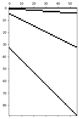
hplot = HierarchicalPlot(S=S_df, tags=tags)
hplot.plot_summing_matrix()
```
## 1. Installing HierarchicalForecast
We assume you have StatsForecast and HierarchicalForecast already
installed, if not check this guide for instructions on how to install
HierarchicalForecast.
```python theme={null}
!pip install hierarchicalforecast statsforecast datasetsforecast
```
```python theme={null}
import os
import numpy as np
import pandas as pd
import matplotlib.pyplot as plt
from statsforecast.core import StatsForecast
from statsforecast.models import AutoARIMA, Naive
from hierarchicalforecast.core import HierarchicalReconciliation
from hierarchicalforecast.methods import BottomUp, TopDown, MinTrace, ERM
from hierarchicalforecast.utils import is_strictly_hierarchical
from hierarchicalforecast.utils import HierarchicalPlot, CodeTimer
from datasetsforecast.hierarchical import HierarchicalData, HierarchicalInfo
```
## 2. Preparing TourismL Dataset
### 2.1 Read Hierarchical Dataset
```python theme={null}
# ['Labour', 'Traffic', 'TourismSmall', 'TourismLarge', 'Wiki2']
dataset = 'TourismSmall' # 'TourismLarge'
verbose = True
intervals_method = 'bootstrap'
LEVEL = np.arange(0, 100, 2)
```
```python theme={null}
with CodeTimer('Read and Parse data ', verbose):
print(f'{dataset}')
if not os.path.exists('./data'):
os.makedirs('./data')
dataset_info = HierarchicalInfo[dataset]
Y_df, S_df, tags = HierarchicalData.load(directory=f'./data/{dataset}', group=dataset)
Y_df['ds'] = pd.to_datetime(Y_df['ds'])
# Train/Test Splits
horizon = dataset_info.horizon
seasonality = dataset_info.seasonality
Y_test_df = Y_df.groupby('unique_id', as_index=False).tail(horizon)
Y_train_df = Y_df.drop(Y_test_df.index)
S_df = S_df.reset_index(names="unique_id")
```
```text theme={null}
TourismSmall
Code block 'Read and Parse data ' took: 0.00653 seconds
```
```python theme={null}
dataset_info.seasonality
```
```text theme={null}
4
```
```python theme={null}
hplot = HierarchicalPlot(S=S_df, tags=tags)
hplot.plot_summing_matrix()
```
 ```python theme={null}
Y_train_df
```
| | unique\_id | ds | y |
| ---- | -------------- | ---------- | ----- |
| 0 | total | 1998-03-31 | 84503 |
| 1 | total | 1998-06-30 | 65312 |
| 2 | total | 1998-09-30 | 72753 |
| 3 | total | 1998-12-31 | 70880 |
| 4 | total | 1999-03-31 | 86893 |
| ... | ... | ... | ... |
| 3191 | nt-oth-noncity | 2003-12-31 | 132 |
| 3192 | nt-oth-noncity | 2004-03-31 | 12 |
| 3193 | nt-oth-noncity | 2004-06-30 | 40 |
| 3194 | nt-oth-noncity | 2004-09-30 | 186 |
| 3195 | nt-oth-noncity | 2004-12-31 | 144 |
### 2.2 StatsForecast’s Base Predictions
This cell computes the base predictions `Y_hat_df` for all the series in
`Y_df` using StatsForecast’s `AutoARIMA`. Additionally we obtain
insample predictions `Y_fitted_df` for the methods that require them.
```python theme={null}
with CodeTimer('Fit/Predict Model ', verbose):
# Read to avoid unnecesary AutoARIMA computation
yhat_file = f'./data/{dataset}/Y_hat.csv'
yfitted_file = f'./data/{dataset}/Y_fitted.csv'
if os.path.exists(yhat_file):
Y_hat_df = pd.read_csv(yhat_file, parse_dates=['ds'])
Y_fitted_df = pd.read_csv(yfitted_file, parse_dates=['ds'])
else:
fcst = StatsForecast(
models=[AutoARIMA(season_length=seasonality)],
fallback_model=[Naive()],
freq=dataset_info.freq,
n_jobs=-1
)
Y_hat_df = fcst.forecast(df=Y_train_df, h=horizon, fitted=True, level=LEVEL)
Y_fitted_df = fcst.forecast_fitted_values()
Y_hat_df.to_csv(yhat_file, index=False)
Y_fitted_df.to_csv(yfitted_file, index=False)
```
## 3. Reconcile Predictions
```python theme={null}
with CodeTimer('Reconcile Predictions ', verbose):
if is_strictly_hierarchical(S=S_df.drop(columns="unique_id").values.astype(np.float32), tags={key: S_df["unique_id"].isin(val).values.nonzero()[0] for key, val in tags.items()}):
reconcilers = [
BottomUp(),
TopDown(method='average_proportions'),
TopDown(method='proportion_averages'),
MinTrace(method='ols'),
MinTrace(method='wls_var'),
MinTrace(method='mint_shrink'),
ERM(method='closed'),
]
else:
reconcilers = [
BottomUp(),
MinTrace(method='ols'),
MinTrace(method='wls_var'),
MinTrace(method='mint_shrink'),
ERM(method='closed'),
]
hrec = HierarchicalReconciliation(reconcilers=reconcilers)
Y_rec_df = hrec.bootstrap_reconcile(Y_hat_df=Y_hat_df,
Y_df=Y_fitted_df,
S_df=S_df, tags=tags,
level=LEVEL,
intervals_method=intervals_method,
num_samples=10,
num_seeds=10)
Y_rec_df = Y_rec_df.merge(Y_test_df, on=['unique_id', 'ds'], how="left")
```
```text theme={null}
Code block 'Reconcile Predictions ' took: 7.49314 seconds
```
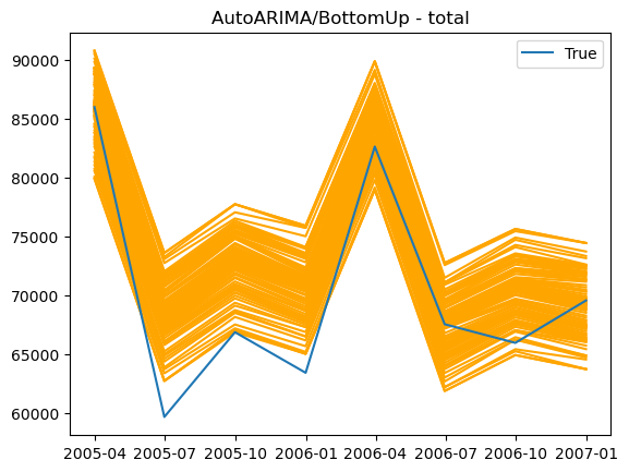
Qualitative evaluation, of parsed quantiles
```python theme={null}
unique_id = "total"
plot_df = Y_rec_df.query("unique_id == @unique_id").groupby(["unique_id", "ds"], as_index=False).mean()
for col in hrec.level_names['AutoARIMA/BottomUp']:
plt.plot(plot_df["ds"], plot_df[col], color="orange")
plt.plot(plot_df["ds"], plot_df["y"], label="True")
plt.title(f"AutoARIMA/BottomUp - {unique_id}")
plt.legend()
```
```python theme={null}
Y_train_df
```
| | unique\_id | ds | y |
| ---- | -------------- | ---------- | ----- |
| 0 | total | 1998-03-31 | 84503 |
| 1 | total | 1998-06-30 | 65312 |
| 2 | total | 1998-09-30 | 72753 |
| 3 | total | 1998-12-31 | 70880 |
| 4 | total | 1999-03-31 | 86893 |
| ... | ... | ... | ... |
| 3191 | nt-oth-noncity | 2003-12-31 | 132 |
| 3192 | nt-oth-noncity | 2004-03-31 | 12 |
| 3193 | nt-oth-noncity | 2004-06-30 | 40 |
| 3194 | nt-oth-noncity | 2004-09-30 | 186 |
| 3195 | nt-oth-noncity | 2004-12-31 | 144 |
### 2.2 StatsForecast’s Base Predictions
This cell computes the base predictions `Y_hat_df` for all the series in
`Y_df` using StatsForecast’s `AutoARIMA`. Additionally we obtain
insample predictions `Y_fitted_df` for the methods that require them.
```python theme={null}
with CodeTimer('Fit/Predict Model ', verbose):
# Read to avoid unnecesary AutoARIMA computation
yhat_file = f'./data/{dataset}/Y_hat.csv'
yfitted_file = f'./data/{dataset}/Y_fitted.csv'
if os.path.exists(yhat_file):
Y_hat_df = pd.read_csv(yhat_file, parse_dates=['ds'])
Y_fitted_df = pd.read_csv(yfitted_file, parse_dates=['ds'])
else:
fcst = StatsForecast(
models=[AutoARIMA(season_length=seasonality)],
fallback_model=[Naive()],
freq=dataset_info.freq,
n_jobs=-1
)
Y_hat_df = fcst.forecast(df=Y_train_df, h=horizon, fitted=True, level=LEVEL)
Y_fitted_df = fcst.forecast_fitted_values()
Y_hat_df.to_csv(yhat_file, index=False)
Y_fitted_df.to_csv(yfitted_file, index=False)
```
## 3. Reconcile Predictions
```python theme={null}
with CodeTimer('Reconcile Predictions ', verbose):
if is_strictly_hierarchical(S=S_df.drop(columns="unique_id").values.astype(np.float32), tags={key: S_df["unique_id"].isin(val).values.nonzero()[0] for key, val in tags.items()}):
reconcilers = [
BottomUp(),
TopDown(method='average_proportions'),
TopDown(method='proportion_averages'),
MinTrace(method='ols'),
MinTrace(method='wls_var'),
MinTrace(method='mint_shrink'),
ERM(method='closed'),
]
else:
reconcilers = [
BottomUp(),
MinTrace(method='ols'),
MinTrace(method='wls_var'),
MinTrace(method='mint_shrink'),
ERM(method='closed'),
]
hrec = HierarchicalReconciliation(reconcilers=reconcilers)
Y_rec_df = hrec.bootstrap_reconcile(Y_hat_df=Y_hat_df,
Y_df=Y_fitted_df,
S_df=S_df, tags=tags,
level=LEVEL,
intervals_method=intervals_method,
num_samples=10,
num_seeds=10)
Y_rec_df = Y_rec_df.merge(Y_test_df, on=['unique_id', 'ds'], how="left")
```
```text theme={null}
Code block 'Reconcile Predictions ' took: 7.49314 seconds
```
Qualitative evaluation, of parsed quantiles
```python theme={null}
unique_id = "total"
plot_df = Y_rec_df.query("unique_id == @unique_id").groupby(["unique_id", "ds"], as_index=False).mean()
for col in hrec.level_names['AutoARIMA/BottomUp']:
plt.plot(plot_df["ds"], plot_df[col], color="orange")
plt.plot(plot_df["ds"], plot_df["y"], label="True")
plt.title(f"AutoARIMA/BottomUp - {unique_id}")
plt.legend()
```
 ## 4. Evaluation
```python theme={null}
from utilsforecast.losses import scaled_crps, msse
from hierarchicalforecast.evaluation import evaluate
from functools import partial
```
```python theme={null}
with CodeTimer('Evaluate Models CRPS and MSSE ', verbose):
metrics_seeds = []
for seed in Y_rec_df.seed.unique():
df_seed = Y_rec_df.query("seed == @seed")
metrics_seed = evaluate(df = df_seed,
tags = tags,
metrics = [scaled_crps,
partial(msse, seasonality=4)],
models= hrec.level_names.keys(),
level = LEVEL,
train_df = Y_train_df,
)
metrics_seed['seed'] = seed
metrics_seeds.append(metrics_seed)
metrics_seeds = pd.concat(metrics_seeds)
metrics_mean = metrics_seeds.groupby(["level", "metric"], as_index=False).mean()
metrics_std = metrics_seeds.groupby(["level", "metric"], as_index=False).std()
results = metrics_mean[hrec.level_names.keys()].round(3).astype(str) + "±" + metrics_std[hrec.level_names.keys()].round(4).astype(str)
results.insert(0, "metric", metrics_mean["metric"])
results.insert(0, "level", metrics_mean["level"])
results.sort_values(by=["metric", "level"])
```
```text theme={null}
Code block 'Evaluate Models CRPS and MSSE ' took: 4.25192 seconds
```
| | level | metric | AutoARIMA/BottomUp | AutoARIMA/TopDown\_method-average\_proportions | AutoARIMA/TopDown\_method-proportion\_averages | AutoARIMA/MinTrace\_method-ols | AutoARIMA/MinTrace\_method-wls\_var | AutoARIMA/MinTrace\_method-mint\_shrink | AutoARIMA/ERM\_method-closed\_lambda\_reg-0.01 |
| - | --------------------------------- | ------------ | ------------------ | ---------------------------------------------- | ---------------------------------------------- | ------------------------------ | ----------------------------------- | --------------------------------------- | ---------------------------------------------- |
| 0 | Country | msse | 1.777±0.0 | 2.488±0.0 | 2.488±0.0 | 2.752±0.0 | 2.569±0.0 | 2.775±0.0 | 3.427±0.0 |
| 2 | Country/Purpose | msse | 1.726±0.0 | 3.181±0.0 | 3.169±0.0 | 2.184±0.0 | 1.876±0.0 | 1.96±0.0 | 3.067±0.0 |
| 4 | Country/Purpose/State | msse | 0.881±0.0 | 1.657±0.0 | 1.652±0.0 | 0.98±0.0 | 0.857±0.0 | 0.867±0.0 | 1.559±0.0 |
| 6 | Country/Purpose/State/CityNonCity | msse | 0.95±0.0 | 1.271±0.0 | 1.269±0.0 | 1.033±0.0 | 0.903±0.0 | 0.912±0.0 | 1.635±0.0 |
| 8 | Overall | msse | 0.973±0.0 | 1.492±0.0 | 1.488±0.0 | 1.087±0.0 | 0.951±0.0 | 0.966±0.0 | 1.695±0.0 |
| 1 | Country | scaled\_crps | 0.043±0.0009 | 0.048±0.0006 | 0.048±0.0006 | 0.05±0.0006 | 0.051±0.0006 | 0.053±0.0006 | 0.054±0.0009 |
| 3 | Country/Purpose | scaled\_crps | 0.077±0.001 | 0.114±0.0003 | 0.112±0.0004 | 0.09±0.0013 | 0.087±0.0009 | 0.089±0.0009 | 0.106±0.0013 |
| 5 | Country/Purpose/State | scaled\_crps | 0.165±0.0009 | 0.249±0.0004 | 0.247±0.0004 | 0.18±0.0018 | 0.169±0.0009 | 0.169±0.0008 | 0.231±0.0021 |
| 7 | Country/Purpose/State/CityNonCity | scaled\_crps | 0.218±0.0013 | 0.289±0.0004 | 0.286±0.0004 | 0.228±0.0018 | 0.217±0.0013 | 0.218±0.0011 | 0.302±0.0033 |
| 9 | Overall | scaled\_crps | 0.193±0.0011 | 0.266±0.0004 | 0.263±0.0004 | 0.205±0.0017 | 0.194±0.0011 | 0.195±0.0009 | 0.268±0.0027 |
## References
* [Syama Sundar Rangapuram, Lucien D Werner, Konstantinos Benidis,
Pedro Mercado, Jan Gasthaus, Tim Januschowski. (2021). "End-to-End
Learning of Coherent Probabilistic Forecasts for Hierarchical Time
Series". Proceedings of the 38th International Conference on Machine
Learning
(ICML).](https://proceedings.mlr.press/v139/rangapuram21a.html)
* [Kin G. Olivares, O. Nganba Meetei, Ruijun Ma, Rohan Reddy, Mengfei
Cao, Lee Dicker (2022). “Probabilistic Hierarchical Forecasting with
Deep Poisson Mixtures”. Submitted to the International Journal
Forecasting, Working paper available at
arxiv.](https://arxiv.org/pdf/2110.13179.pdf)
## 4. Evaluation
```python theme={null}
from utilsforecast.losses import scaled_crps, msse
from hierarchicalforecast.evaluation import evaluate
from functools import partial
```
```python theme={null}
with CodeTimer('Evaluate Models CRPS and MSSE ', verbose):
metrics_seeds = []
for seed in Y_rec_df.seed.unique():
df_seed = Y_rec_df.query("seed == @seed")
metrics_seed = evaluate(df = df_seed,
tags = tags,
metrics = [scaled_crps,
partial(msse, seasonality=4)],
models= hrec.level_names.keys(),
level = LEVEL,
train_df = Y_train_df,
)
metrics_seed['seed'] = seed
metrics_seeds.append(metrics_seed)
metrics_seeds = pd.concat(metrics_seeds)
metrics_mean = metrics_seeds.groupby(["level", "metric"], as_index=False).mean()
metrics_std = metrics_seeds.groupby(["level", "metric"], as_index=False).std()
results = metrics_mean[hrec.level_names.keys()].round(3).astype(str) + "±" + metrics_std[hrec.level_names.keys()].round(4).astype(str)
results.insert(0, "metric", metrics_mean["metric"])
results.insert(0, "level", metrics_mean["level"])
results.sort_values(by=["metric", "level"])
```
```text theme={null}
Code block 'Evaluate Models CRPS and MSSE ' took: 4.25192 seconds
```
| | level | metric | AutoARIMA/BottomUp | AutoARIMA/TopDown\_method-average\_proportions | AutoARIMA/TopDown\_method-proportion\_averages | AutoARIMA/MinTrace\_method-ols | AutoARIMA/MinTrace\_method-wls\_var | AutoARIMA/MinTrace\_method-mint\_shrink | AutoARIMA/ERM\_method-closed\_lambda\_reg-0.01 |
| - | --------------------------------- | ------------ | ------------------ | ---------------------------------------------- | ---------------------------------------------- | ------------------------------ | ----------------------------------- | --------------------------------------- | ---------------------------------------------- |
| 0 | Country | msse | 1.777±0.0 | 2.488±0.0 | 2.488±0.0 | 2.752±0.0 | 2.569±0.0 | 2.775±0.0 | 3.427±0.0 |
| 2 | Country/Purpose | msse | 1.726±0.0 | 3.181±0.0 | 3.169±0.0 | 2.184±0.0 | 1.876±0.0 | 1.96±0.0 | 3.067±0.0 |
| 4 | Country/Purpose/State | msse | 0.881±0.0 | 1.657±0.0 | 1.652±0.0 | 0.98±0.0 | 0.857±0.0 | 0.867±0.0 | 1.559±0.0 |
| 6 | Country/Purpose/State/CityNonCity | msse | 0.95±0.0 | 1.271±0.0 | 1.269±0.0 | 1.033±0.0 | 0.903±0.0 | 0.912±0.0 | 1.635±0.0 |
| 8 | Overall | msse | 0.973±0.0 | 1.492±0.0 | 1.488±0.0 | 1.087±0.0 | 0.951±0.0 | 0.966±0.0 | 1.695±0.0 |
| 1 | Country | scaled\_crps | 0.043±0.0009 | 0.048±0.0006 | 0.048±0.0006 | 0.05±0.0006 | 0.051±0.0006 | 0.053±0.0006 | 0.054±0.0009 |
| 3 | Country/Purpose | scaled\_crps | 0.077±0.001 | 0.114±0.0003 | 0.112±0.0004 | 0.09±0.0013 | 0.087±0.0009 | 0.089±0.0009 | 0.106±0.0013 |
| 5 | Country/Purpose/State | scaled\_crps | 0.165±0.0009 | 0.249±0.0004 | 0.247±0.0004 | 0.18±0.0018 | 0.169±0.0009 | 0.169±0.0008 | 0.231±0.0021 |
| 7 | Country/Purpose/State/CityNonCity | scaled\_crps | 0.218±0.0013 | 0.289±0.0004 | 0.286±0.0004 | 0.228±0.0018 | 0.217±0.0013 | 0.218±0.0011 | 0.302±0.0033 |
| 9 | Overall | scaled\_crps | 0.193±0.0011 | 0.266±0.0004 | 0.263±0.0004 | 0.205±0.0017 | 0.194±0.0011 | 0.195±0.0009 | 0.268±0.0027 |
## References
* [Syama Sundar Rangapuram, Lucien D Werner, Konstantinos Benidis,
Pedro Mercado, Jan Gasthaus, Tim Januschowski. (2021). "End-to-End
Learning of Coherent Probabilistic Forecasts for Hierarchical Time
Series". Proceedings of the 38th International Conference on Machine
Learning
(ICML).](https://proceedings.mlr.press/v139/rangapuram21a.html)
* [Kin G. Olivares, O. Nganba Meetei, Ruijun Ma, Rohan Reddy, Mengfei
Cao, Lee Dicker (2022). “Probabilistic Hierarchical Forecasting with
Deep Poisson Mixtures”. Submitted to the International Journal
Forecasting, Working paper available at
arxiv.](https://arxiv.org/pdf/2110.13179.pdf)