> ## Documentation Index
> Fetch the complete documentation index at: https://nixtlaverse.nixtla.io/llms.txt
> Use this file to discover all available pages before exploring further.
# Introduction
> Introduction to Hierarchical Forecasting using `HierarchicalForecast`
You can run these experiments using CPU or GPU with Google Colab.
 ## 1. Hierarchical Series
In many applications, a set of time series is hierarchically organized.
Examples include the presence of geographic levels, products, or
categories that define different types of aggregations.
In such scenarios, forecasters are often required to provide predictions
for all disaggregate and aggregate series. A natural desire is for those
predictions to be **“coherent”**, that is, for the bottom series to add
up precisely to the forecasts of the aggregated series.
## 1. Hierarchical Series
In many applications, a set of time series is hierarchically organized.
Examples include the presence of geographic levels, products, or
categories that define different types of aggregations.
In such scenarios, forecasters are often required to provide predictions
for all disaggregate and aggregate series. A natural desire is for those
predictions to be **“coherent”**, that is, for the bottom series to add
up precisely to the forecasts of the aggregated series.
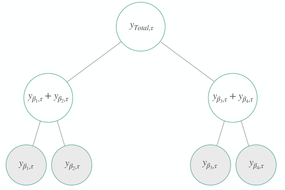 The above figure shows a simple hierarchical structure where we have
four bottom-level series, two middle-level series, and the top level
representing the total aggregation. Its hierarchical aggregations or
coherency constraints are:
$$
y_{\mathrm{Total},\tau} = y_{\beta_{1},\tau}+y_{\beta_{2},\tau}+y_{\beta_{3},\tau}+y_{\beta_{4},\tau}
\qquad \qquad \qquad \qquad \qquad \\
\mathbf{y}_{[a],\tau}=\left[y_{\mathrm{Total},\tau},\; y_{\beta_{1},\tau}+y_{\beta_{2},\tau},\;y_{\beta_{3},\tau}+y_{\beta_{4},\tau}\right]^{\intercal}
\qquad
\mathbf{y}_{[b],\tau}=\left[ y_{\beta_{1},\tau},\; y_{\beta_{2},\tau},\; y_{\beta_{3},\tau},\; y_{\beta_{4},\tau} \right]^{\intercal}
$$
Luckily these constraints can be compactly expressed with the following
matrices:
$$
\mathbf{S}_{[a,b][b]}
=
\begin{bmatrix}
\mathbf{A}_{\mathrm{[a][b]}} \\
\\
\\
\mathbf{I}_{\mathrm{[b][b]}} \\
\\
\end{bmatrix}
=
\begin{bmatrix}
1 & 1 & 1 & 1 \\
1 & 1 & 0 & 0 \\
0 & 0 & 1 & 1 \\
1 & 0 & 0 & 0 \\
0 & 1 & 0 & 0 \\
0 & 0 & 1 & 0 \\
0 & 0 & 0 & 1 \\
\end{bmatrix}
$$
where $\mathbf{A}_{[a,b][b]}$ aggregates the bottom series to the upper
levels, and $\mathbf{I}_{\mathrm{[b][b]}}$ is an identity matrix. The
representation of the hierarchical series is then:
$$
\mathbf{y}_{[a,b],\tau} = \mathbf{S}_{[a,b][b]} \mathbf{y}_{[b],\tau}
$$
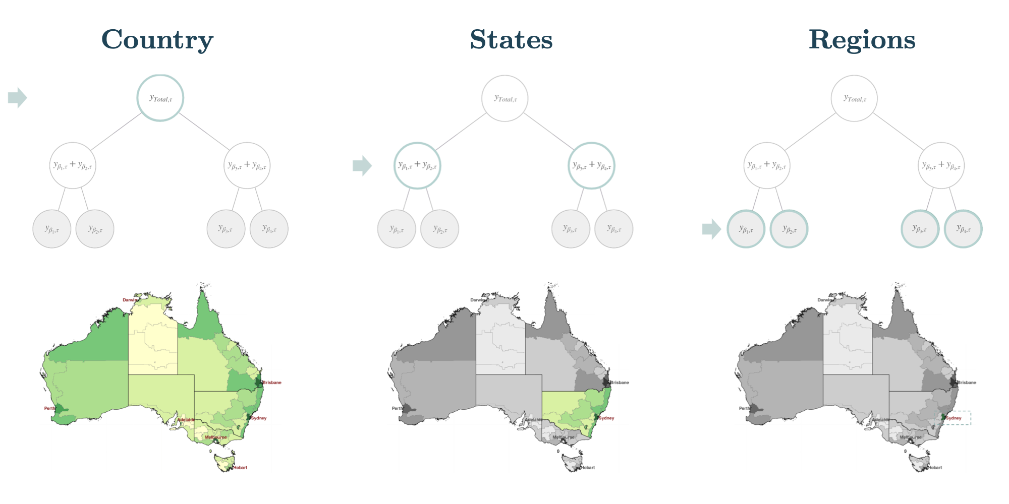
To visualize an example, in Figure 2, one can think of the hierarchical
time series structure levels to represent different geographical
aggregations. For example, in Figure 2, the top level is the total
aggregation of series within a country, the middle level being its
states and the bottom level its regions.
The above figure shows a simple hierarchical structure where we have
four bottom-level series, two middle-level series, and the top level
representing the total aggregation. Its hierarchical aggregations or
coherency constraints are:
$$
y_{\mathrm{Total},\tau} = y_{\beta_{1},\tau}+y_{\beta_{2},\tau}+y_{\beta_{3},\tau}+y_{\beta_{4},\tau}
\qquad \qquad \qquad \qquad \qquad \\
\mathbf{y}_{[a],\tau}=\left[y_{\mathrm{Total},\tau},\; y_{\beta_{1},\tau}+y_{\beta_{2},\tau},\;y_{\beta_{3},\tau}+y_{\beta_{4},\tau}\right]^{\intercal}
\qquad
\mathbf{y}_{[b],\tau}=\left[ y_{\beta_{1},\tau},\; y_{\beta_{2},\tau},\; y_{\beta_{3},\tau},\; y_{\beta_{4},\tau} \right]^{\intercal}
$$
Luckily these constraints can be compactly expressed with the following
matrices:
$$
\mathbf{S}_{[a,b][b]}
=
\begin{bmatrix}
\mathbf{A}_{\mathrm{[a][b]}} \\
\\
\\
\mathbf{I}_{\mathrm{[b][b]}} \\
\\
\end{bmatrix}
=
\begin{bmatrix}
1 & 1 & 1 & 1 \\
1 & 1 & 0 & 0 \\
0 & 0 & 1 & 1 \\
1 & 0 & 0 & 0 \\
0 & 1 & 0 & 0 \\
0 & 0 & 1 & 0 \\
0 & 0 & 0 & 1 \\
\end{bmatrix}
$$
where $\mathbf{A}_{[a,b][b]}$ aggregates the bottom series to the upper
levels, and $\mathbf{I}_{\mathrm{[b][b]}}$ is an identity matrix. The
representation of the hierarchical series is then:
$$
\mathbf{y}_{[a,b],\tau} = \mathbf{S}_{[a,b][b]} \mathbf{y}_{[b],\tau}
$$
To visualize an example, in Figure 2, one can think of the hierarchical
time series structure levels to represent different geographical
aggregations. For example, in Figure 2, the top level is the total
aggregation of series within a country, the middle level being its
states and the bottom level its regions.
 ## 2. Hierarchical Forecast
To achieve **“coherency”**, most statistical solutions to the
hierarchical forecasting challenge implement a two-stage reconciliation
process.
1. First, we obtain a set of the base forecast
$\mathbf{\hat{y}}_{[a,b],\tau}$
2. Later, we reconcile them into coherent forecasts
$\mathbf{\tilde{y}}_{[a,b],\tau}$.
Most hierarchical reconciliation methods can be expressed by the
following transformations:
$$
\tilde{\mathbf{y}}_{[a,b],\tau} = \mathbf{S}_{[a,b][b]} \mathbf{P}_{[b][a,b]} \hat{\mathbf{y}}_{[a,b],\tau}
$$
The HierarchicalForecast library offers a Python collection of
reconciliation methods, datasets, evaluation and visualization tools for
the task. Among its available reconciliation methods we have `BottomUp`,
`TopDown`, `MiddleOut`, `MinTrace`, `ERM`. Among its probabilistic
coherent methods we have `Normality`, `Bootstrap`, `PERMBU`.
## 3. Minimal Example
```python theme={null}
!pip install hierarchicalforecast statsforecast datasetsforecast
```
### Wrangling Data
```python theme={null}
import numpy as np
import pandas as pd
```
We are going to create a synthetic data set to illustrate a hierarchical
time series structure like the one in Figure 1.
We will create a two level structure with four bottom series where
aggregations of the series are self evident.
```python theme={null}
# Create Figure 1. synthetic bottom data
ds = pd.date_range(start="2000-01-01", end="2000-08-01", freq="MS")
y_base = np.arange(1, 9)
r1 = y_base * (10 ** 1)
r2 = y_base * (10 ** 1)
r3 = y_base * (10 ** 2)
r4 = y_base * (10 ** 2)
ys = np.concatenate([r1, r2, r3, r4])
ds = np.tile(ds, 4)
unique_ids = ["r1"] * 8 + ["r2"] * 8 + ["r3"] * 8 + ["r4"] * 8
top_level = "Australia"
middle_level = ["State1"] * 16 + ["State2"] * 16
bottom_level = unique_ids
bottom_df = dict(
ds=ds,
top_level=top_level,
middle_level=middle_level,
bottom_level=bottom_level,
y=ys,
)
bottom_df = pd.DataFrame(bottom_df)
bottom_df.groupby("bottom_level").head(2)
```
The previously introduced hierarchical series $\mathbf{y}_{[a,b]\tau}$
is captured within the `Y_hier_df` dataframe.
The aggregation constraints matrix $\mathbf{S}_{[a][b]}$ is captured
within the `S_df` dataframe.
Finally `tags` contains a dictionary of lists within `Y_hier_df`
composing each hierarchical level, for example the `tags['top_level']`
contains `Australia`’s aggregated series index.
```python theme={null}
from hierarchicalforecast.utils import aggregate
```
```python theme={null}
# Create hierarchical structure and constraints
hierarchy_levels = [
["top_level"],
["top_level", "middle_level"],
["top_level", "middle_level", "bottom_level"],
]
Y_hier_df, S_df, tags = aggregate(df=bottom_df, spec=hierarchy_levels)
print("S_df.shape", S_df.shape)
print("Y_hier_df.shape", Y_hier_df.shape)
print("tags['top_level']", tags["top_level"])
```
```python theme={null}
Y_hier_df.groupby("unique_id").head(2)
```
```python theme={null}
S_df
```
### Base Predictions
Next, we compute the *base forecast* for each time series using the
`naive` model. Observe that `Y_hat_df` contains the forecasts but they
are not coherent.
```python theme={null}
from statsforecast.models import Naive
from statsforecast.core import StatsForecast
```
```python theme={null}
# Split train/test sets
Y_test_df = Y_hier_df.groupby("unique_id", as_index=False).tail(4)
Y_train_df = Y_hier_df.drop(Y_test_df.index)
# Compute base Naive predictions
# Careful identifying correct data freq, this data monthly 'M'
fcst = StatsForecast(models=[Naive()], freq="MS", n_jobs=-1)
Y_hat_df = fcst.forecast(df=Y_train_df, h=4, fitted=True)
Y_fitted_df = fcst.forecast_fitted_values()
```
### Reconciliation
```python theme={null}
from hierarchicalforecast.methods import BottomUp
from hierarchicalforecast.core import HierarchicalReconciliation
```
```python theme={null}
# You can select a reconciler from our collection
reconcilers = [BottomUp()] # MinTrace(method='mint_shrink')
hrec = HierarchicalReconciliation(reconcilers=reconcilers)
Y_rec_df = hrec.reconcile(Y_hat_df=Y_hat_df, Y_df=Y_fitted_df, S_df=S_df, tags=tags)
Y_rec_df.groupby("unique_id").head(2)
```
## References
* [Hyndman, R.J., & Athanasopoulos, G. (2021). “Forecasting:
principles and practice, 3rd edition: Chapter 11: Forecasting
hierarchical and grouped series.”. OTexts: Melbourne, Australia.
OTexts.com/fpp3 Accessed on July
2022.](https://otexts.com/fpp3/hierarchical.html)
## 2. Hierarchical Forecast
To achieve **“coherency”**, most statistical solutions to the
hierarchical forecasting challenge implement a two-stage reconciliation
process.
1. First, we obtain a set of the base forecast
$\mathbf{\hat{y}}_{[a,b],\tau}$
2. Later, we reconcile them into coherent forecasts
$\mathbf{\tilde{y}}_{[a,b],\tau}$.
Most hierarchical reconciliation methods can be expressed by the
following transformations:
$$
\tilde{\mathbf{y}}_{[a,b],\tau} = \mathbf{S}_{[a,b][b]} \mathbf{P}_{[b][a,b]} \hat{\mathbf{y}}_{[a,b],\tau}
$$
The HierarchicalForecast library offers a Python collection of
reconciliation methods, datasets, evaluation and visualization tools for
the task. Among its available reconciliation methods we have `BottomUp`,
`TopDown`, `MiddleOut`, `MinTrace`, `ERM`. Among its probabilistic
coherent methods we have `Normality`, `Bootstrap`, `PERMBU`.
## 3. Minimal Example
```python theme={null}
!pip install hierarchicalforecast statsforecast datasetsforecast
```
### Wrangling Data
```python theme={null}
import numpy as np
import pandas as pd
```
We are going to create a synthetic data set to illustrate a hierarchical
time series structure like the one in Figure 1.
We will create a two level structure with four bottom series where
aggregations of the series are self evident.
```python theme={null}
# Create Figure 1. synthetic bottom data
ds = pd.date_range(start="2000-01-01", end="2000-08-01", freq="MS")
y_base = np.arange(1, 9)
r1 = y_base * (10 ** 1)
r2 = y_base * (10 ** 1)
r3 = y_base * (10 ** 2)
r4 = y_base * (10 ** 2)
ys = np.concatenate([r1, r2, r3, r4])
ds = np.tile(ds, 4)
unique_ids = ["r1"] * 8 + ["r2"] * 8 + ["r3"] * 8 + ["r4"] * 8
top_level = "Australia"
middle_level = ["State1"] * 16 + ["State2"] * 16
bottom_level = unique_ids
bottom_df = dict(
ds=ds,
top_level=top_level,
middle_level=middle_level,
bottom_level=bottom_level,
y=ys,
)
bottom_df = pd.DataFrame(bottom_df)
bottom_df.groupby("bottom_level").head(2)
```
The previously introduced hierarchical series $\mathbf{y}_{[a,b]\tau}$
is captured within the `Y_hier_df` dataframe.
The aggregation constraints matrix $\mathbf{S}_{[a][b]}$ is captured
within the `S_df` dataframe.
Finally `tags` contains a dictionary of lists within `Y_hier_df`
composing each hierarchical level, for example the `tags['top_level']`
contains `Australia`’s aggregated series index.
```python theme={null}
from hierarchicalforecast.utils import aggregate
```
```python theme={null}
# Create hierarchical structure and constraints
hierarchy_levels = [
["top_level"],
["top_level", "middle_level"],
["top_level", "middle_level", "bottom_level"],
]
Y_hier_df, S_df, tags = aggregate(df=bottom_df, spec=hierarchy_levels)
print("S_df.shape", S_df.shape)
print("Y_hier_df.shape", Y_hier_df.shape)
print("tags['top_level']", tags["top_level"])
```
```python theme={null}
Y_hier_df.groupby("unique_id").head(2)
```
```python theme={null}
S_df
```
### Base Predictions
Next, we compute the *base forecast* for each time series using the
`naive` model. Observe that `Y_hat_df` contains the forecasts but they
are not coherent.
```python theme={null}
from statsforecast.models import Naive
from statsforecast.core import StatsForecast
```
```python theme={null}
# Split train/test sets
Y_test_df = Y_hier_df.groupby("unique_id", as_index=False).tail(4)
Y_train_df = Y_hier_df.drop(Y_test_df.index)
# Compute base Naive predictions
# Careful identifying correct data freq, this data monthly 'M'
fcst = StatsForecast(models=[Naive()], freq="MS", n_jobs=-1)
Y_hat_df = fcst.forecast(df=Y_train_df, h=4, fitted=True)
Y_fitted_df = fcst.forecast_fitted_values()
```
### Reconciliation
```python theme={null}
from hierarchicalforecast.methods import BottomUp
from hierarchicalforecast.core import HierarchicalReconciliation
```
```python theme={null}
# You can select a reconciler from our collection
reconcilers = [BottomUp()] # MinTrace(method='mint_shrink')
hrec = HierarchicalReconciliation(reconcilers=reconcilers)
Y_rec_df = hrec.reconcile(Y_hat_df=Y_hat_df, Y_df=Y_fitted_df, S_df=S_df, tags=tags)
Y_rec_df.groupby("unique_id").head(2)
```
## References
* [Hyndman, R.J., & Athanasopoulos, G. (2021). “Forecasting:
principles and practice, 3rd edition: Chapter 11: Forecasting
hierarchical and grouped series.”. OTexts: Melbourne, Australia.
OTexts.com/fpp3 Accessed on July
2022.](https://otexts.com/fpp3/hierarchical.html)
* [Orcutt, G.H., Watts, H.W., & Edwards, J.B.(1968). Data aggregation
and information loss. The American Economic Review, 58 ,
773(787).](http://www.jstor.org/stable/1815532)
* [Disaggregation methods to expedite product line forecasting.
Journal of Forecasting, 9 , 233–254.
doi:10.1002/for.3980090304.](https://onlinelibrary.wiley.com/doi/abs/10.1002/for.3980090304)
* [Wickramasuriya, S. L., Athanasopoulos, G., & Hyndman, R. J. (2019).
"Optimal forecast reconciliation for hierarchical and grouped time
series through trace minimization". Journal of the American
Statistical Association, 114 , 804–819.
doi:10.1080/01621459.2018.1448825.](https://robjhyndman.com/publications/mint/)
* [Ben Taieb, S., & Koo, B. (2019). Regularized regression for
hierarchical forecasting without unbiasedness conditions. In
Proceedings of the 25th ACM SIGKDD International Conference on
Knowledge Discovery & Data Mining KDD ’19 (p. 1337(1347). New York,
NY, USA: Association for Computing
Machinery.](https://doi.org/10.1145/3292500.3330976)