> ## Documentation Index
> Fetch the complete documentation index at: https://nixtlaverse.nixtla.io/llms.txt
> Use this file to discover all available pages before exploring further.
# PERMBU
 In many cases, only the time series at the lowest level of the
hierarchies (bottom time series) are available. `HierarchicalForecast`
has tools to create time series for all hierarchies and also allows you
to calculate prediction intervals for all hierarchies. In this notebook
we will see how to do it.
```python theme={null}
!pip install hierarchicalforecast statsforecast
```
```python theme={null}
import pandas as pd
# compute base forecast no coherent
from statsforecast.models import AutoARIMA
from statsforecast.core import StatsForecast
#obtain hierarchical reconciliation methods and evaluation
from hierarchicalforecast.methods import BottomUp, MinTrace
from hierarchicalforecast.utils import aggregate, HierarchicalPlot
from hierarchicalforecast.core import HierarchicalReconciliation
```
## Aggregate bottom time series
In this example we will use the
[Tourism](https://otexts.com/fpp3/tourism.html) dataset from the
[Forecasting: Principles and Practice](https://otexts.com/fpp3/) book.
The dataset only contains the time series at the lowest level, so we
need to create the time series for all hierarchies.
```python theme={null}
Y_df = pd.read_csv('https://raw.githubusercontent.com/Nixtla/transfer-learning-time-series/main/datasets/tourism.csv')
Y_df = Y_df.rename({'Trips': 'y', 'Quarter': 'ds'}, axis=1)
Y_df.insert(0, 'Country', 'Australia')
Y_df = Y_df[['Country', 'Region', 'State', 'Purpose', 'ds', 'y']]
Y_df['ds'] = Y_df['ds'].str.replace(r'(\d+) (Q\d)', r'\1-\2', regex=True)
Y_df['ds'] = pd.PeriodIndex(Y_df["ds"], freq='Q').to_timestamp()
Y_df.head()
```
| | Country | Region | State | Purpose | ds | y |
| - | --------- | -------- | --------------- | -------- | ---------- | ---------- |
| 0 | Australia | Adelaide | South Australia | Business | 1998-01-01 | 135.077690 |
| 1 | Australia | Adelaide | South Australia | Business | 1998-04-01 | 109.987316 |
| 2 | Australia | Adelaide | South Australia | Business | 1998-07-01 | 166.034687 |
| 3 | Australia | Adelaide | South Australia | Business | 1998-10-01 | 127.160464 |
| 4 | Australia | Adelaide | South Australia | Business | 1999-01-01 | 137.448533 |
The dataset can be grouped in the following strictly hierarchical
structure.
```python theme={null}
spec = [
['Country'],
['Country', 'State'],
['Country', 'State', 'Region']
]
```
Using the `aggregate` function from `HierarchicalForecast` we can get
the full set of time series.
```python theme={null}
Y_df, S_df, tags = aggregate(df=Y_df, spec=spec)
```
```python theme={null}
Y_df.head()
```
| | unique\_id | ds | y |
| - | ---------- | ---------- | ------------ |
| 0 | Australia | 1998-01-01 | 23182.197269 |
| 1 | Australia | 1998-04-01 | 20323.380067 |
| 2 | Australia | 1998-07-01 | 19826.640511 |
| 3 | Australia | 1998-10-01 | 20830.129891 |
| 4 | Australia | 1999-01-01 | 22087.353380 |
```python theme={null}
S_df.iloc[:5, :5]
```
| | unique\_id | Australia/ACT/Canberra | Australia/New South Wales/Blue Mountains | Australia/New South Wales/Capital Country | Australia/New South Wales/Central Coast |
| - | ---------------------------- | ---------------------- | ---------------------------------------- | ----------------------------------------- | --------------------------------------- |
| 0 | Australia | 1.0 | 1.0 | 1.0 | 1.0 |
| 1 | Australia/ACT | 1.0 | 0.0 | 0.0 | 0.0 |
| 2 | Australia/New South Wales | 0.0 | 1.0 | 1.0 | 1.0 |
| 3 | Australia/Northern Territory | 0.0 | 0.0 | 0.0 | 0.0 |
| 4 | Australia/Queensland | 0.0 | 0.0 | 0.0 | 0.0 |
```python theme={null}
tags['Country/State']
```
```text theme={null}
array(['Australia/ACT', 'Australia/New South Wales',
'Australia/Northern Territory', 'Australia/Queensland',
'Australia/South Australia', 'Australia/Tasmania',
'Australia/Victoria', 'Australia/Western Australia'], dtype=object)
```
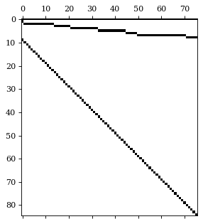
We can visualize the `S` matrix and the data using the
`HierarchicalPlot` class as follows.
```python theme={null}
hplot = HierarchicalPlot(S=S_df, tags=tags)
```
```python theme={null}
hplot.plot_summing_matrix()
```
In many cases, only the time series at the lowest level of the
hierarchies (bottom time series) are available. `HierarchicalForecast`
has tools to create time series for all hierarchies and also allows you
to calculate prediction intervals for all hierarchies. In this notebook
we will see how to do it.
```python theme={null}
!pip install hierarchicalforecast statsforecast
```
```python theme={null}
import pandas as pd
# compute base forecast no coherent
from statsforecast.models import AutoARIMA
from statsforecast.core import StatsForecast
#obtain hierarchical reconciliation methods and evaluation
from hierarchicalforecast.methods import BottomUp, MinTrace
from hierarchicalforecast.utils import aggregate, HierarchicalPlot
from hierarchicalforecast.core import HierarchicalReconciliation
```
## Aggregate bottom time series
In this example we will use the
[Tourism](https://otexts.com/fpp3/tourism.html) dataset from the
[Forecasting: Principles and Practice](https://otexts.com/fpp3/) book.
The dataset only contains the time series at the lowest level, so we
need to create the time series for all hierarchies.
```python theme={null}
Y_df = pd.read_csv('https://raw.githubusercontent.com/Nixtla/transfer-learning-time-series/main/datasets/tourism.csv')
Y_df = Y_df.rename({'Trips': 'y', 'Quarter': 'ds'}, axis=1)
Y_df.insert(0, 'Country', 'Australia')
Y_df = Y_df[['Country', 'Region', 'State', 'Purpose', 'ds', 'y']]
Y_df['ds'] = Y_df['ds'].str.replace(r'(\d+) (Q\d)', r'\1-\2', regex=True)
Y_df['ds'] = pd.PeriodIndex(Y_df["ds"], freq='Q').to_timestamp()
Y_df.head()
```
| | Country | Region | State | Purpose | ds | y |
| - | --------- | -------- | --------------- | -------- | ---------- | ---------- |
| 0 | Australia | Adelaide | South Australia | Business | 1998-01-01 | 135.077690 |
| 1 | Australia | Adelaide | South Australia | Business | 1998-04-01 | 109.987316 |
| 2 | Australia | Adelaide | South Australia | Business | 1998-07-01 | 166.034687 |
| 3 | Australia | Adelaide | South Australia | Business | 1998-10-01 | 127.160464 |
| 4 | Australia | Adelaide | South Australia | Business | 1999-01-01 | 137.448533 |
The dataset can be grouped in the following strictly hierarchical
structure.
```python theme={null}
spec = [
['Country'],
['Country', 'State'],
['Country', 'State', 'Region']
]
```
Using the `aggregate` function from `HierarchicalForecast` we can get
the full set of time series.
```python theme={null}
Y_df, S_df, tags = aggregate(df=Y_df, spec=spec)
```
```python theme={null}
Y_df.head()
```
| | unique\_id | ds | y |
| - | ---------- | ---------- | ------------ |
| 0 | Australia | 1998-01-01 | 23182.197269 |
| 1 | Australia | 1998-04-01 | 20323.380067 |
| 2 | Australia | 1998-07-01 | 19826.640511 |
| 3 | Australia | 1998-10-01 | 20830.129891 |
| 4 | Australia | 1999-01-01 | 22087.353380 |
```python theme={null}
S_df.iloc[:5, :5]
```
| | unique\_id | Australia/ACT/Canberra | Australia/New South Wales/Blue Mountains | Australia/New South Wales/Capital Country | Australia/New South Wales/Central Coast |
| - | ---------------------------- | ---------------------- | ---------------------------------------- | ----------------------------------------- | --------------------------------------- |
| 0 | Australia | 1.0 | 1.0 | 1.0 | 1.0 |
| 1 | Australia/ACT | 1.0 | 0.0 | 0.0 | 0.0 |
| 2 | Australia/New South Wales | 0.0 | 1.0 | 1.0 | 1.0 |
| 3 | Australia/Northern Territory | 0.0 | 0.0 | 0.0 | 0.0 |
| 4 | Australia/Queensland | 0.0 | 0.0 | 0.0 | 0.0 |
```python theme={null}
tags['Country/State']
```
```text theme={null}
array(['Australia/ACT', 'Australia/New South Wales',
'Australia/Northern Territory', 'Australia/Queensland',
'Australia/South Australia', 'Australia/Tasmania',
'Australia/Victoria', 'Australia/Western Australia'], dtype=object)
```
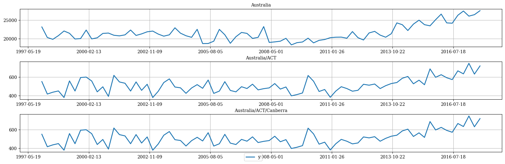
We can visualize the `S` matrix and the data using the
`HierarchicalPlot` class as follows.
```python theme={null}
hplot = HierarchicalPlot(S=S_df, tags=tags)
```
```python theme={null}
hplot.plot_summing_matrix()
```
 ```python theme={null}
hplot.plot_hierarchically_linked_series(
bottom_series='Australia/ACT/Canberra',
Y_df=Y_df
)
```
```python theme={null}
hplot.plot_hierarchically_linked_series(
bottom_series='Australia/ACT/Canberra',
Y_df=Y_df
)
```
 ### Split Train/Test sets
We use the final two years (8 quarters) as test set.
```python theme={null}
Y_test_df = Y_df.groupby('unique_id', as_index=False).tail(8)
Y_train_df = Y_df.drop(Y_test_df.index)
```
```python theme={null}
Y_train_df.groupby('unique_id').size()
```
```text theme={null}
unique_id
Australia 72
Australia/ACT 72
Australia/ACT/Canberra 72
Australia/New South Wales 72
Australia/New South Wales/Blue Mountains 72
..
Australia/Western Australia/Australia's Coral Coast 72
Australia/Western Australia/Australia's Golden Outback 72
Australia/Western Australia/Australia's North West 72
Australia/Western Australia/Australia's South West 72
Australia/Western Australia/Experience Perth 72
Length: 85, dtype: int64
```
## Computing base forecasts
The following cell computes the **base forecasts** for each time series
in `Y_df` using the `AutoARIMA` and model. Observe that `Y_hat_df`
contains the forecasts but they are not coherent. To reconcile the
prediction intervals we need to calculate the uncoherent intervals using
the `level` argument of `StatsForecast`.
```python theme={null}
fcst = StatsForecast(models=[AutoARIMA(season_length=4)],
freq='QS', n_jobs=-1)
Y_hat_df = fcst.forecast(df=Y_train_df, h=8, fitted=True, level=[80, 90])
Y_fitted_df = fcst.forecast_fitted_values()
```
## Reconcile forecasts and compute prediction intervals using PERMBU
The following cell makes the previous forecasts coherent using the
`HierarchicalReconciliation` class. In this example we use `BottomUp`
and `MinTrace`. If you want to calculate prediction intervals, you have
to use the `level` argument as follows and also
`intervals_method='permbu'`.
```python theme={null}
reconcilers = [
BottomUp(),
MinTrace(method='mint_shrink'),
MinTrace(method='ols')
]
hrec = HierarchicalReconciliation(reconcilers=reconcilers)
Y_rec_df = hrec.reconcile(Y_hat_df=Y_hat_df, Y_df=Y_fitted_df,
S_df=S_df, tags=tags,
level=[80, 90], intervals_method='permbu')
```
The dataframe `Y_rec_df` contains the reconciled forecasts.
```python theme={null}
Y_rec_df.head()
```
| | unique\_id | ds | AutoARIMA | AutoARIMA-lo-90 | AutoARIMA-lo-80 | AutoARIMA-hi-80 | AutoARIMA-hi-90 | AutoARIMA/BottomUp | AutoARIMA/BottomUp-lo-90 | AutoARIMA/BottomUp-lo-80 | ... | AutoARIMA/MinTrace\_method-mint\_shrink | AutoARIMA/MinTrace\_method-mint\_shrink-lo-90 | AutoARIMA/MinTrace\_method-mint\_shrink-lo-80 | AutoARIMA/MinTrace\_method-mint\_shrink-hi-80 | AutoARIMA/MinTrace\_method-mint\_shrink-hi-90 | AutoARIMA/MinTrace\_method-ols | AutoARIMA/MinTrace\_method-ols-lo-90 | AutoARIMA/MinTrace\_method-ols-lo-80 | AutoARIMA/MinTrace\_method-ols-hi-80 | AutoARIMA/MinTrace\_method-ols-hi-90 |
| - | ---------- | ---------- | ------------ | --------------- | --------------- | --------------- | --------------- | ------------------ | ------------------------ | ------------------------ | --- | --------------------------------------- | --------------------------------------------- | --------------------------------------------- | --------------------------------------------- | --------------------------------------------- | ------------------------------ | ------------------------------------ | ------------------------------------ | ------------------------------------ | ------------------------------------ |
| 0 | Australia | 2016-01-01 | 26212.553553 | 24705.948180 | 25038.715077 | 27386.392029 | 27719.158927 | 24955.501571 | 24143.056131 | 24387.230200 | ... | 25413.657606 | 24705.682710 | 24905.677772 | 25928.334367 | 26050.232961 | 26142.818016 | 25525.081721 | 25656.537995 | 26606.345032 | 26832.423921 |
| 1 | Australia | 2016-04-01 | 25033.667125 | 23337.267588 | 23711.954696 | 26355.379554 | 26730.066662 | 23421.312868 | 22762.045247 | 22904.087197 | ... | 24058.906411 | 23486.828548 | 23627.152623 | 24659.405484 | 24847.778503 | 24946.338649 | 24297.061230 | 24434.805048 | 25535.549040 | 25640.659918 |
| 2 | Australia | 2016-07-01 | 24507.027198 | 22640.028798 | 23052.396413 | 25961.657983 | 26374.025599 | 22807.706826 | 22065.402373 | 22223.120404 | ... | 23438.863893 | 22672.658701 | 22888.299153 | 23971.724733 | 24179.548677 | 24407.245003 | 23712.841797 | 23834.054327 | 25027.073615 | 25189.869286 |
| 3 | Australia | 2016-10-01 | 25598.928613 | 23575.665243 | 24022.547410 | 27175.309816 | 27622.191983 | 23471.845870 | 22677.593575 | 22892.328939 | ... | 24322.049398 | 23619.419712 | 23682.803746 | 24847.299228 | 25028.345572 | 25496.855604 | 24740.210465 | 24923.560783 | 26094.250414 | 26273.617732 |
| 4 | Australia | 2017-01-01 | 26982.576796 | 24669.535238 | 25180.421285 | 28784.732308 | 29295.618354 | 24668.735931 | 23760.842072 | 23964.283124 | ... | 25520.163549 | 24720.304392 | 24910.106650 | 26170.552678 | 26347.181903 | 26853.231907 | 26045.213677 | 26149.753374 | 27502.499674 | 27733.985566 |
## Plot forecasts
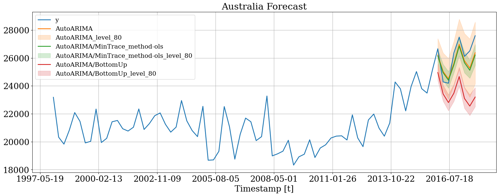
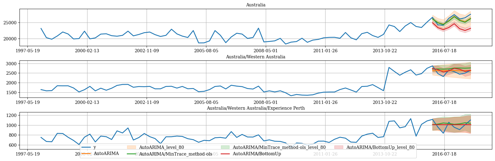
Then we can plot the probabilist forecasts using the following function.
```python theme={null}
plot_df = Y_df.merge(Y_rec_df, on=['unique_id', 'ds'], how="outer")
```
### Plot single time series
```python theme={null}
hplot.plot_series(
series='Australia',
Y_df=plot_df,
models=['y', 'AutoARIMA',
'AutoARIMA/MinTrace_method-ols',
'AutoARIMA/BottomUp'
],
level=[80]
)
```
### Split Train/Test sets
We use the final two years (8 quarters) as test set.
```python theme={null}
Y_test_df = Y_df.groupby('unique_id', as_index=False).tail(8)
Y_train_df = Y_df.drop(Y_test_df.index)
```
```python theme={null}
Y_train_df.groupby('unique_id').size()
```
```text theme={null}
unique_id
Australia 72
Australia/ACT 72
Australia/ACT/Canberra 72
Australia/New South Wales 72
Australia/New South Wales/Blue Mountains 72
..
Australia/Western Australia/Australia's Coral Coast 72
Australia/Western Australia/Australia's Golden Outback 72
Australia/Western Australia/Australia's North West 72
Australia/Western Australia/Australia's South West 72
Australia/Western Australia/Experience Perth 72
Length: 85, dtype: int64
```
## Computing base forecasts
The following cell computes the **base forecasts** for each time series
in `Y_df` using the `AutoARIMA` and model. Observe that `Y_hat_df`
contains the forecasts but they are not coherent. To reconcile the
prediction intervals we need to calculate the uncoherent intervals using
the `level` argument of `StatsForecast`.
```python theme={null}
fcst = StatsForecast(models=[AutoARIMA(season_length=4)],
freq='QS', n_jobs=-1)
Y_hat_df = fcst.forecast(df=Y_train_df, h=8, fitted=True, level=[80, 90])
Y_fitted_df = fcst.forecast_fitted_values()
```
## Reconcile forecasts and compute prediction intervals using PERMBU
The following cell makes the previous forecasts coherent using the
`HierarchicalReconciliation` class. In this example we use `BottomUp`
and `MinTrace`. If you want to calculate prediction intervals, you have
to use the `level` argument as follows and also
`intervals_method='permbu'`.
```python theme={null}
reconcilers = [
BottomUp(),
MinTrace(method='mint_shrink'),
MinTrace(method='ols')
]
hrec = HierarchicalReconciliation(reconcilers=reconcilers)
Y_rec_df = hrec.reconcile(Y_hat_df=Y_hat_df, Y_df=Y_fitted_df,
S_df=S_df, tags=tags,
level=[80, 90], intervals_method='permbu')
```
The dataframe `Y_rec_df` contains the reconciled forecasts.
```python theme={null}
Y_rec_df.head()
```
| | unique\_id | ds | AutoARIMA | AutoARIMA-lo-90 | AutoARIMA-lo-80 | AutoARIMA-hi-80 | AutoARIMA-hi-90 | AutoARIMA/BottomUp | AutoARIMA/BottomUp-lo-90 | AutoARIMA/BottomUp-lo-80 | ... | AutoARIMA/MinTrace\_method-mint\_shrink | AutoARIMA/MinTrace\_method-mint\_shrink-lo-90 | AutoARIMA/MinTrace\_method-mint\_shrink-lo-80 | AutoARIMA/MinTrace\_method-mint\_shrink-hi-80 | AutoARIMA/MinTrace\_method-mint\_shrink-hi-90 | AutoARIMA/MinTrace\_method-ols | AutoARIMA/MinTrace\_method-ols-lo-90 | AutoARIMA/MinTrace\_method-ols-lo-80 | AutoARIMA/MinTrace\_method-ols-hi-80 | AutoARIMA/MinTrace\_method-ols-hi-90 |
| - | ---------- | ---------- | ------------ | --------------- | --------------- | --------------- | --------------- | ------------------ | ------------------------ | ------------------------ | --- | --------------------------------------- | --------------------------------------------- | --------------------------------------------- | --------------------------------------------- | --------------------------------------------- | ------------------------------ | ------------------------------------ | ------------------------------------ | ------------------------------------ | ------------------------------------ |
| 0 | Australia | 2016-01-01 | 26212.553553 | 24705.948180 | 25038.715077 | 27386.392029 | 27719.158927 | 24955.501571 | 24143.056131 | 24387.230200 | ... | 25413.657606 | 24705.682710 | 24905.677772 | 25928.334367 | 26050.232961 | 26142.818016 | 25525.081721 | 25656.537995 | 26606.345032 | 26832.423921 |
| 1 | Australia | 2016-04-01 | 25033.667125 | 23337.267588 | 23711.954696 | 26355.379554 | 26730.066662 | 23421.312868 | 22762.045247 | 22904.087197 | ... | 24058.906411 | 23486.828548 | 23627.152623 | 24659.405484 | 24847.778503 | 24946.338649 | 24297.061230 | 24434.805048 | 25535.549040 | 25640.659918 |
| 2 | Australia | 2016-07-01 | 24507.027198 | 22640.028798 | 23052.396413 | 25961.657983 | 26374.025599 | 22807.706826 | 22065.402373 | 22223.120404 | ... | 23438.863893 | 22672.658701 | 22888.299153 | 23971.724733 | 24179.548677 | 24407.245003 | 23712.841797 | 23834.054327 | 25027.073615 | 25189.869286 |
| 3 | Australia | 2016-10-01 | 25598.928613 | 23575.665243 | 24022.547410 | 27175.309816 | 27622.191983 | 23471.845870 | 22677.593575 | 22892.328939 | ... | 24322.049398 | 23619.419712 | 23682.803746 | 24847.299228 | 25028.345572 | 25496.855604 | 24740.210465 | 24923.560783 | 26094.250414 | 26273.617732 |
| 4 | Australia | 2017-01-01 | 26982.576796 | 24669.535238 | 25180.421285 | 28784.732308 | 29295.618354 | 24668.735931 | 23760.842072 | 23964.283124 | ... | 25520.163549 | 24720.304392 | 24910.106650 | 26170.552678 | 26347.181903 | 26853.231907 | 26045.213677 | 26149.753374 | 27502.499674 | 27733.985566 |
## Plot forecasts
Then we can plot the probabilist forecasts using the following function.
```python theme={null}
plot_df = Y_df.merge(Y_rec_df, on=['unique_id', 'ds'], how="outer")
```
### Plot single time series
```python theme={null}
hplot.plot_series(
series='Australia',
Y_df=plot_df,
models=['y', 'AutoARIMA',
'AutoARIMA/MinTrace_method-ols',
'AutoARIMA/BottomUp'
],
level=[80]
)
```
 ### Plot hierarchichally linked time series
```python theme={null}
hplot.plot_hierarchically_linked_series(
bottom_series='Australia/Western Australia/Experience Perth',
Y_df=plot_df,
models=['y', 'AutoARIMA', 'AutoARIMA/MinTrace_method-ols', 'AutoARIMA/BottomUp'],
level=[80]
)
```
### Plot hierarchichally linked time series
```python theme={null}
hplot.plot_hierarchically_linked_series(
bottom_series='Australia/Western Australia/Experience Perth',
Y_df=plot_df,
models=['y', 'AutoARIMA', 'AutoARIMA/MinTrace_method-ols', 'AutoARIMA/BottomUp'],
level=[80]
)
```
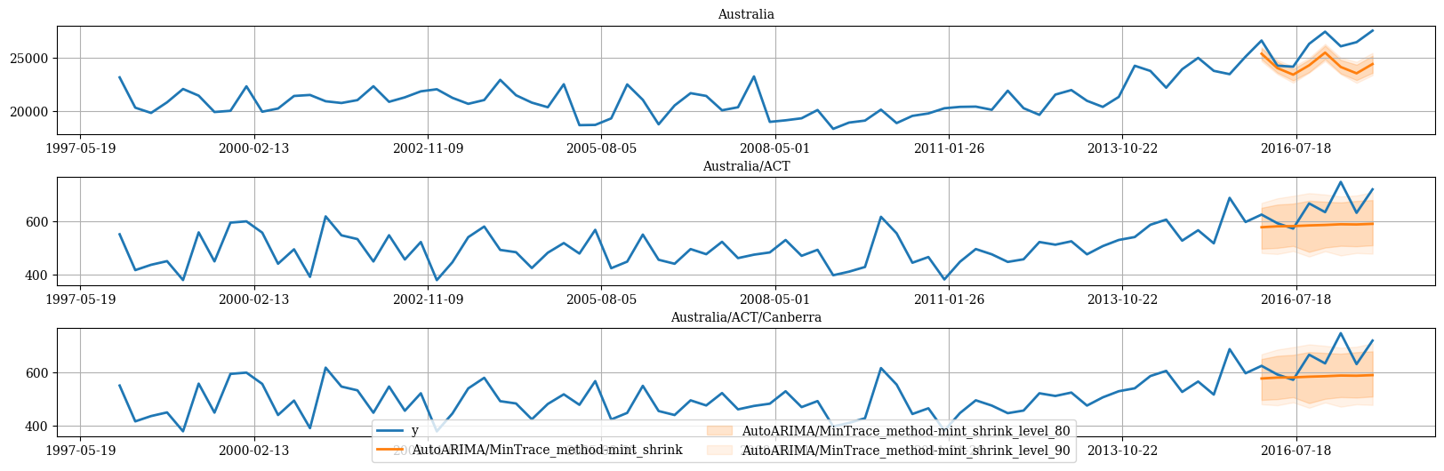
 ```python theme={null}
# ACT only has Canberra
hplot.plot_hierarchically_linked_series(
bottom_series='Australia/ACT/Canberra',
Y_df=plot_df,
models=['y', 'AutoARIMA/MinTrace_method-mint_shrink'],
level=[80, 90]
)
```
```python theme={null}
# ACT only has Canberra
hplot.plot_hierarchically_linked_series(
bottom_series='Australia/ACT/Canberra',
Y_df=plot_df,
models=['y', 'AutoARIMA/MinTrace_method-mint_shrink'],
level=[80, 90]
)
```
 ### References
* [Hyndman, R.J., & Athanasopoulos, G. (2021). “Forecasting:
principles and practice, 3rd edition: Chapter 11: Forecasting
hierarchical and grouped series.”. OTexts: Melbourne, Australia.
OTexts.com/fpp3 Accessed on July
2022.](https://otexts.com/fpp3/hierarchical.html)
* [Shanika L. Wickramasuriya, George Athanasopoulos, and Rob J.
Hyndman. Optimal forecast reconciliation for hierarchical and
grouped time series through trace minimization.Journal of the
American Statistical Association, 114(526):804–819, 2019. doi:
10.1080/01621459.2018.1448825. URL
https://robjhyndman.com/publications/mint/.](https://robjhyndman.com/publications/mint/)
### References
* [Hyndman, R.J., & Athanasopoulos, G. (2021). “Forecasting:
principles and practice, 3rd edition: Chapter 11: Forecasting
hierarchical and grouped series.”. OTexts: Melbourne, Australia.
OTexts.com/fpp3 Accessed on July
2022.](https://otexts.com/fpp3/hierarchical.html)
* [Shanika L. Wickramasuriya, George Athanasopoulos, and Rob J.
Hyndman. Optimal forecast reconciliation for hierarchical and
grouped time series through trace minimization.Journal of the
American Statistical Association, 114(526):804–819, 2019. doi:
10.1080/01621459.2018.1448825. URL
https://robjhyndman.com/publications/mint/.](https://robjhyndman.com/publications/mint/)